Electronic Supplement to
The Source of the 30 October 1930, M_w 5.8, Senigallia (Central Italy) Earthquake: A Convergent Solution from Instrumental, Macroseismic and Geological Data

by Paola Vannoli, Gianfranco Vannucci, Fabrizio Bernardi, Barbara Palombo, and Graziano Ferrari

This electronic supplement contains methods, data, and elaborations that support and make more transparent the seismotectonic characterization of the 30 October 1930 Senigallia earthquake. In particular, it provides a short description of the method used for moment tensor computation; all the available focal mechanisms (Table S1); the list of the available stations, with specification of which were used for hypocenter and moment tensor computation (Table S3); maps of seismic flux showing areas of larger energy release; and detailed maps of the uncertainties for each realization of the macroseismic epicenter (Figure S2).

---

Short Description of the Moment Tensor Computation Method (from Bernardi et al., unpublished manuscript)

The early mechanical and electromagnetic seismographs, respectively recorded on smoked and photographic paper, were significantly different from modern digital broadband seismometers. The main differences include the frequency range sensitivity, the magnification, the quality of the recordings, the clock precision, and the size of the recordings. The following is a brief description of these differences and of their implications.

1. Frequency Range Sensitivity: Digital broadband seismometers are generally sensitive to a wide range of frequency (generally between 0.01 and 10 Hz) in which the instrument response is mainly flat. In contrast, mechanical seismometers (e.g., Wiechert) are sensitive to a very narrow frequency range (centered around 0.1 Hz), whereas electromagnetic seismometers (e.g., Galitzin) are sensitive to a frequency range in the order of 0.04–0.1 Hz.
2. Magnification: the ground velocity magnification of modern broadband seismometers is very large (1×10¹⁰ and over), whereas it is between 50–200 and 200–800 around the instrument natural frequency for mechanical and electromagnetic seismometers, respectively (Bernardi et al., 2005). The limited frequency range sensitivity and low magnification of the early mechanical and electromagnetic seismometers implies that some seismic phases may not be well resolved in the seismogram.
3. Quality of the Recordings: mechanical and electromagnetic seismometers saturate faster than broadband seismometers, because their dynamic range is smaller than that of digital instruments. Most of the quality limitations on early seismometers arise from the characteristics of the recording support (smoked and photographic paper) and of the mechanics of the recording device. When strong ground motion occurs, the recording nib starts moving fast. Because of aerodynamic effects, the nib may lose grip on the paper, resulting in a poorly visible trace and in the loss of some details of the waveform.
4. Clock Precision: In 1930 the clock time of recording systems was synchronized with a radio signal only in a few observatories and seismic stations worldwide; hence, for most of the observatories, the clock synchronization uncertainty was larger than a few seconds.
5. Size of the Recording: The low speed of the recording drum (15 or 30 mm/min) of early seismographs made the waveform recordings more sensitive to variations of the recording drum speed. Even when the clock synchronization was very accurate, small variations of the drum speed combined with the small size of the recordings may have introduced distortions into the phase arrival times.

The short- and middle-period sensitivity of the seismometers implies the use of short and middle periods for waveform modeling. Earth models at regional and global scales for such periods are generally not available. This would require calibrating a source-path velocity model for each earthquake and for each source–receiver configuration. In addition, amplitudes and phase velocities may exhibit distortions caused by a combination of conditions 3 and 4.

Because of the problems described above, we approached the moment tensor computation in the frequency spectrum domain rather than in the time domain. Spectrum amplitudes are less sensitive to heterogeneities in the Earth model than phase velocities. We inverted the waveforms and synthetic seismograms into the frequency spectrum domain, and then used the P-wave first arrival polarities to constrain the P and T axes. This approach is similar to the method proposed by Zaradnik et al. (2001), which uses higher frequencies recorded at local distances from digital seismometers, thus requiring a very dense network with stations close to the source. Unfortunately, the datasets available for early instrumental historical earthquakes, such as the one described here from 1930, generally include only few and geographically sparse recorded seismograms.

Our proposed approach is similar to the method described by Okal and Reymond (2003). They used it in the inversion of the power spectrum within the 0.01–0.003 Hz frequency range for a very large earthquake (M_w 8.6), making the contribution of crustal and mantle structures negligible. Unfortunately, the sensitivity of all mechanical and of most electromagnetic seismometers is low, which implies that their method is suitable for large earthquakes recorded at teleseismic distance but not for moderate earthquake recorded at regional distance, as in our case.

Because our dataset of observed data is sparse, we adopted a scheme of linear forward modeling: we kept the epicenter and the depth fixed and looked for the best-fitting amplitude spectra between the normalized observed and the synthetic seismograms while varying the source model. This method (Bernardi et al., unpublished manuscript) is composed of (1) a Green’s function generated for each source-recording station path by normal mode summation (Woodhouse, 1988) using the SURF96 algorithm (Hermann, 2004; see Data and Resources); (2) a simple Monte Carlo method for generating synthetic seismograms convolving the Green’s function with a set of 5000 randomly computed synthetic moment tensors (MTs), previously calculated and stored into a library; (3) the computation of theoretical P-wave polarities at each station for each synthetic MT; (4) the radial and transverse components of the synthetic seismogram, which are rotated into the seismometer reference system and then convolved with the instrument transfer function, computed from the instrument constants; (5) the assessment of the normalized variance between synthetic and observed power spectra amplitude, searching for the solution among the minimum variance and the best fit between observed and theoretical P-wave polarities; and (6) the assessment of the seismic moment M₀ for the best MT solution from power spectra amplitudes.

---

Seismic Flux

To outline the tectonic strain pattern, we derived the seismic flux as in Serpelloni et al. (2007), using the seismicity supplied by the 2011 Catalogo Parametrico dei Terremoti Italiani (CPTI11), International Seismological Centre (ISC), Catalogo Strumentale dei Terremoti Italiani (CSTI), Catalogo della Sismicità Italiana (CSI), Bollettino Sismico Italiano (BSI) and Italian Seismological Instrumental and parametric Data-basE (ISIDE) catalogs and taking advantage from various available empirical calibrations (Gasperini et al., 2013a,b; Lolli et al., 2014). These allowed us to re-evaluate homogeneous M_w of events and equivalent scalar seismic moment (M₀) using the Hanks and Kanamori (1979) relation. In particular, we selected crustal earthquakes (i.e., events located between the Earth surface and the Moho). The Moho depth was computed over a 0.1° × 0.1° grid mesh (Molinari and Morelli, 2011) and for the study area was found to range between 15 and 30 km. We also added 5 km of conservative threshold for the crustal thickness to avoid the loss of significant crustal earthquakes due to uncertainty on their depth. This choice is not critical for the aims of this analysis because all well-located earthquakes are included. Then, using a regular 0.1° × 0.1° grid mesh for each crustal earthquake, we estimated the radius of the seismic crack (i.e., the semi-length of the seismogenic fault derived from the scalar seismic moment of each event) from the standard scaling relationships (Kanamori and Anderson, 1975). We computed the percentage of the seismic crack area (and then of the scalar seismic moment) falling into each cell and cumulated the scalar seismic moment for each cell. This provides the seismic moment released (in dyn·cm) per unit area (in km²) and per year. Finally, we interpolated the values found for each cell to obtain a map of the coseismic energy released in time and in space (i.e., the seismic flux) and to overcome possible gaps in the seismicity. This approach has the advantage of averaging out the earthquake location uncertainties by interpolating the data so as to obtain a fairly detailed overview of the areas where seismic activity occurred. The seismic flux cannot be considered representative of the whole amplitude of active tectonic strain, yet it represents a qualitative tool to outline its spatial distribution. The qualitative nature of the analysis increases as the considered time interval decreases.

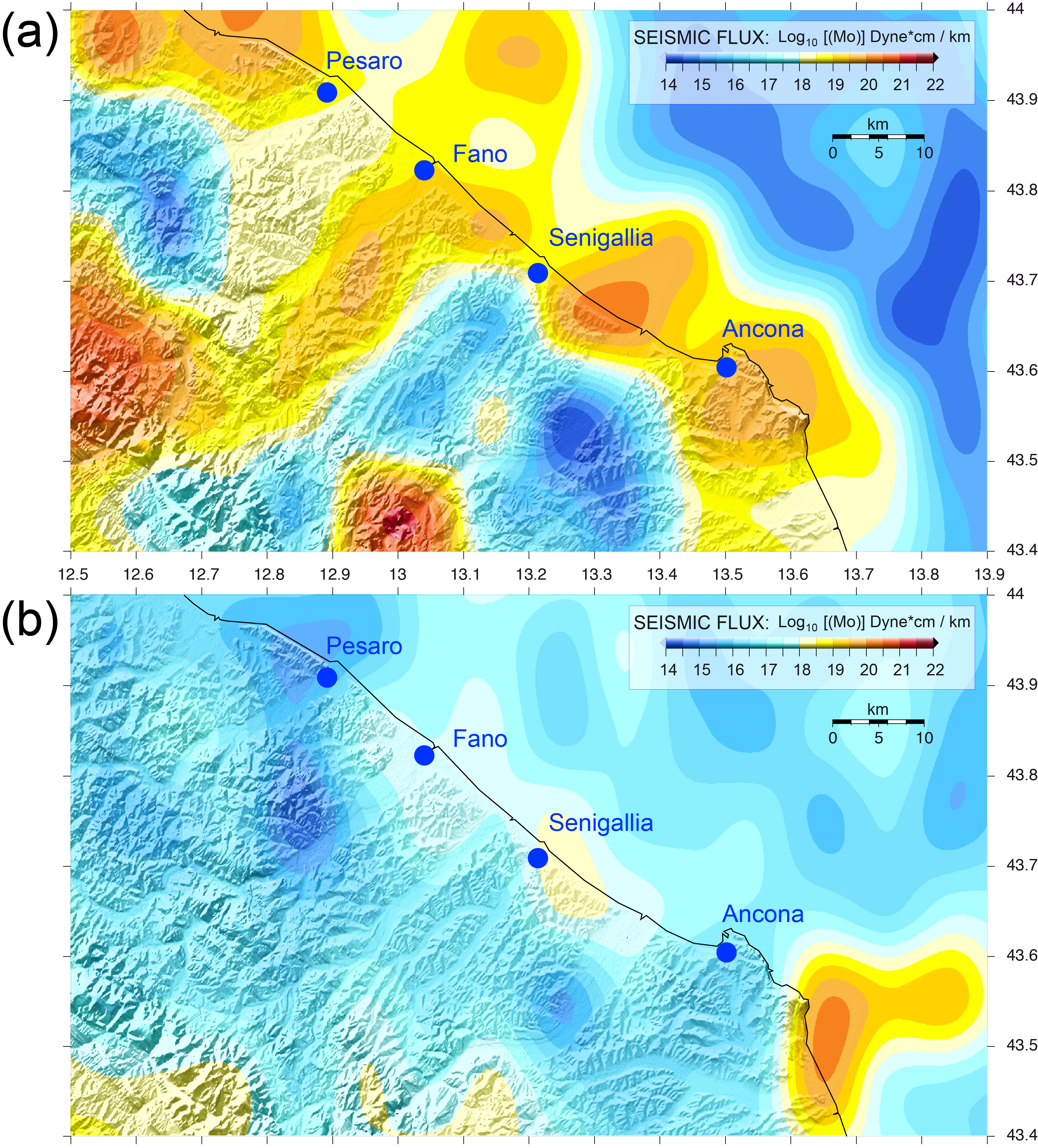
We selected two different time spans: from A.D. 1600 to present (Fig. S1a) and from 1981 to present (Fig. S1b). The threshold of A.D. 1600 allowed us to include the strongest earthquakes of the study area, because the CPTI11 is known to be complete since A.D. 1600 for events larger than M 5.5.

In Figure S1a, although the seismicity outlines the locations of large seismic moment release (with values up to 1×10²² dyn·cm/km²/yr) related to the strongest earthquakes that occurred since A.D. 1600, two spatially continuous subparallel belts with a roughly northwest–southeast orientation (mainly displayed in yellow and orange colors) characterize the study area. These belts delineate the seismically active portion of the crestal part of the Apennines and the coastal seismic zone, which are separated by a region that experiences a significantly lower seismic flux (blue color tones).

In Figure S1b, the seismicity that has occurred since 1981 is generally characterized by lower values of the seismic flux with respect to the 400-year time span since A.D. 1600. Two spots of relatively higher moment release are seen along the coast: one (with values up to 1×10¹⁹ dyn·cm/km²/yr) located to the southeast of Ancona and related to the 21 July 2013 earthquake and to the subsequent aftershocks sequence, and another located slightly southeast of Senigallia. The latter location, which falls close to the macroseismic epicenter of the 1930 earthquake, indicates an active area with relatively higher coseismic flux.

---

Figures

Figure S1. Seismic flux (i.e., the distribution of seismic energy release per unit area and per year in the study area) (a) since A.D. 1600 and (b) since 1981. (See preceding discussion for additional details.)

Figure S2. Epicenters of the 1930 earthquake obtained with all the methods made available by the Boxer code (Gasperini et al., 2010). The figure shows also bootstrap (i.e., empirical) uncertainty ellipses (at 90% of confidence) and normalized percentage density distributions for all the locations of the bootstrap paradata sets (n=240).

---

Tables

Table S1. All the available focal mechanisms and their parameters.

Table S2. Stations not used for hypocentral location.

Table S3. List of the stations not used for the moment tensor computation.

---

Data and Resources

Bollettino Sismico Italiano (BSI) was searched using http://bollettinosismico.rm.ingv.it (last accessed October 2013).

Catalogo della Sismicità Italiana (CSI) v.1.1 was searched using http://csi.rm.ingv.it/ (last accessed October 2013).

Catalogo Parametrico dei Terremoti Italiani (CPTI11; doi: 10.6092/INGV.IT-CPTI11) was searched using http://emidius.mi.ingv.it/CPTI (last accessed July 2014).

Catalogo Strumentale dei Terremoti Italiani (CSTI) v.1.1, was searched using http://gaspy.df.unibo.it/paolo/gndt/Versione1_1/Leggimi.htm (last accessed October 2013).

Earthquake mechanisms of the Mediterranean Area (EMMA), http://ibogfs.df.unibo.it/user2/paolo/www/ATLAS/pages/EMMA_description.htm (last accessed August 2014).

European-Mediterranean Regional Centroid Moment Tensor (RCMT) catalog of INGV from 1997 to 2010 was searched using http://www.bo.ingv.it/RCMT/ (last access, November 2014).

Global Centroid Moment Tensor catalog, from 1976 to May 2010 (GCMT), was searched using http://www.globalcmt.org/CMTfiles.html (last accessed November 2014).

International Seismological Centre Bulletin (ISC) was searched using www.isc.ac.uk (last accessed December 2013).

Italian Seismological Instrumental and parametric Data-basE (ISIDE) was searched using http://iside.rm.ingv.it/iside/standard/index.jsp (last accessed December 2013).

Quick Regional Moment Tensors of INGV was searched using http://autorcmt.bo.ingv.it/quicks.html (last access, November 2014).

Time Domain Moment Tensor (TDMT) catalog of INGV from 2006 to 2013 was searched using http://cnt.rm.ingv.it/tdmt.html (last access, November 2014).

Vannucci G., P. Imprescia, and P. Gasperini (2010). Deliverable Number 2 of the UR2.05 in the INGV-DPC S1 project (2007–2009). INGV-DPC Internal report and database.

---

[ Back ]