|
|
Publications: SRL: Opinion |

January/February 2009
Thirty Years of Confusion around “Scattering Q”?
The past 30 years have seen vast advances in seismic instrumentation, computing infrastructure, and methodology. In particular, an impressive concept of the frequency-dependent attenuation quality, Q(ƒ), was created, followed by a dazzling array of related theories and models. However, revisiting some of its original postulates still shows that theoretical models may have run somewhat ahead of the observational constraints. Many presentations of Q(ƒ) have been influenced by the prevalence of particular models, especially those based on random scattering. This led to the well-known apparent character of Q(ƒ) and excessive complexity of its interpretations, which start from unrealistic assumptions about the wavefield and then justify them in retrospect. To regain clarity, I suggest abandoning the use of Q for scattering and reviewing some of the key datasets in an assumption-free and data-driven manner. Initial efforts in this direction show that frequency-dependent Q may not be nearly as widespread as currently thought. These points are briefly discussed below.
Current Q(ƒ) Paradigm—Inadequate for Structured Earth
In most interpretations of seismic attenuation, the measurements can be reduced to inversion of some time- and frequencyvariant path factor P(t, ƒ) representing the seismic amplitudes from which the effects of the source and receiver have been removed:
| P (t, ƒ) = | G0 (t) e | − | π ƒt Q(ƒ) . |
(1) | |
A well-known fundamental problem is the definition of the geometrical spreading factor, G0(t), which in some cases may also be frequency-dependent. When G0(t) is set from simple theoretical considerations (e.g., G0(t) ∝ t–1 for body waves in a uniform isotropic space) but applied to real data, a frequency-dependent Q arises: Q(ƒ) = Q0 ƒ η. This Q is then typically attributed to random scattering (e.g., Aki 1980) or to rheology.
From discussions with many seismologists, I discovered that it is surprisingly difficult to argue these simple points. The problem seems rooted in the established culture of corroborating models by other models and other authors’ papers, and in a sacred belief in the magic of algorithms and less attention to the data.
However, a big question still remains: What physics and what properties of the Earth do the Q0 and η values, or what combinations of them, really correspond to? These quantities relate to the assumed G0(t) at least as much as to the path effect (Equation 1). Note that when η ≈ 1 (which is often observed), P(t, ƒ) becomes frequency-independent, which means that it is purely geometrical and there is no need to invoke the Q-factor at all. Also, a variation of about ±10% in the geometrical powerlaw exponent could eliminate the frequency- dependent Q in Equation 1 in the typical cases of –0.3 < η < 0.4 (Morozov 2008). Such variations should be common in the observations. Thus, the Q(ƒ) factor in Equation 1, and particularly the “scattering Q,” is based on the definition of G0(t) and simultaneously masks the inaccuracy of this definition.
The scattering theory (e.g., Chernov 1960, 35–57,) does not use Q to represent scattering, which is described by the differential cross-section, turbidity, or the mean free path. Scattering has a different physics from intrinsic attenuation, which implies energy dissipation proportional to the number of wave oscillations (i.e., to the product ft in Equation 1) and not to the travel path length. The scattering quality factor was introduced by Aki (1980) in order to render scattering-related losses similarly to those caused by the intrinsic attenuation. This was convenient, but there the analogy ended. As one can see, the most commonly observed trend of Q increasing with frequency (η > 0) is principally due to Q being the denominator of the relatively weak frequency-dependent exponent in Equation 1. For these reasons, I refer to the Q(ƒ) as defined by Equation 1 as confusing and misleading, and I suggest that its use not be overemphasized.
From discussions with many seismologists, I discovered that it is surprisingly difficult to argue these simple points. The problem seems rooted in the established culture of corroborating models by other models and other authors’ papers, and in a sacred belief in the magic of algorithms and less attention to the data. The argument often degenerates to selecting various G0(t) models and fitting the data. Paradoxically, many people seem to be content with conclusions that, for example, Q(ƒ) equals 360ƒ ½ provided the geometrical spreading equals r−1 (Aki 1980). This of course is the same as saying that the Earth is uniform and structureless but contains random scatterers. If one changes this assumption, which is reasonable to do, the Q(ƒ) formula would change and scatterers may no longer be seen. This uncertainty is also broadly accepted as the apparent character of Q. Yet, despite their subjective and apparent character, interpretations based on the unstable parameters Q0 and η are also common.
An argument often advanced in support of the scattering hypothesis and the frequency-dependent Q in Equation 1 is that such models “work.” However, it is important to understand how inverse modeling works in general. The Q(ƒ) inversion is performed for a complex set of parameters (Q0, η, and sometimes source and site) but by using only limited observations (for example, coda envelope slopes). Such inversions are known as underconstrained, and it is equally known that their principal property is the ability to fit the data but not so much to determine the model. The ability to fit the attenuation-coefficient data still does not prove the scattering hypothesis, despite the suggestions by Aki (1980) repeated by many others. It simply does not disprove it. The data can be fit in other, and, as argued below, better ways. The determination of the Q(ƒ) model actually comes mostly from a priori constraints, which in this case are the assumed geometrical spreading, isotropy, a simple form of the wavefield, etc.
Unambiguous Attenuation Model
After this critique, an unambiguous solution for the Q(ƒ) problem is surprisingly and refreshingly simple: just let the data be the guide! Consider the attenuation coefficient α(ƒ), which is the nominator of the exponent in Equation 1, and explicitly separate its zero-frequency part, denoted by γ = α(0) below:
Derivation of α(ƒ) is an intermediate step of most Q(ƒ) measurements, yet it is never presented because of the assumed α(ƒ) = πƒ /Q(ƒ) relation in Equation 1. However, before making this assumption, one should still examine the dependence of α(ƒ) on the frequency, which can be done by plotting it in a linear frequency scale. The intercept γ then measures the corrected geometrical spreading: G(t) = G0(t)e–γ, and the frequency-dependent part α(ƒ) – α(0) = πƒ/Qe defines the quality factor Qe corresponding to the “effective” attenuation (Morozov 2008). Note that unlike Q(ƒ), Qe is not biased by the zero-frequency (geometrical) part of α(ƒ), and it can therefore be associated with intrinsic and true small-scale scattering.
…exploration seismologists often admit that their predictions are correct in only 25% of the cases, even though they take advantage of well-controlled experiments, vast amounts of data, and a lot more regular and shallower targets…. The domain of earthquake seismology is significantly more complex, and therefore its success rate does not have to be even that high.
In Equation 2, Qe may or may not be frequency-dependent, which is to be established from the data. However, having studied many published examples of different wave types within several frequency bands (Morozov 2008), I still have found no cases where a frequency-dependent Qe would be required! The attenuation coefficient α(ƒ) in Equation 2 shows consistent linear dependencies within the available measurement errors, and the resulting Qe values are significantly (typically, by 2–20 times) higher than Q0.
In a spectacular example, Figure 1A shows the observed broadband frequency-dependent Q–1(ƒ) compiled from Anderson and Given (1982) and Abercrombie (1998). The values of Q–1 exhibit a band-limited increase, which was interpreted as caused by the mantle absorption band (Anderson and Given 1982). However, reconstruction of the α(ƒ) data from these Q–1(ƒ) leads to a different interpretation (Figures 1B–C). Three ranges of linear α(ƒ) dependencies can be recognized, with the linearity within the crustal body-wave band with a nonzero γ > 0 being particularly clear (thick lines and labels in Figure 1). The two breaks in α(ƒ) slopes should be caused by changing wave types and depths of sampling. Given the data scatter, there appear to be no indications of frequency-dependent Qe within these bands. Therefore, instead of frequency-dependent rheological properties of the mantle, the data suggest depth banding of Qe: two low-Q bands within the core and upper mantle and a higher- Qe crust (Figure 1). Also note that the mantle and core modes spread slightly slower (γ < 0 in Figure 1B) but that crustal waves spread slightly faster (γ > 0 in Figure 1C) than predicted by the corresponding geometrical-compensation models. Obviously, the consequences of such a change in the interpretation should be profound.
Finally, skeptics sometimes say that Equation 2 is just another model of Q(ƒ), and therefore there is nothing new to it. Indeed, similarly to Equation 1, this two-parameter relation also describes the observed P(t, ƒ), but with a different interpretational connotation. It focuses on measuring the structure (represented by γ) instead of assuming scattering in a uniform space. This is also the only model independent of the geometrical- spreading assumptions, with stable and portable parameters, and in which the frequency dependence of Q can be examined with confidence. Overall, stable and simple models should be much preferred in the interpretation.
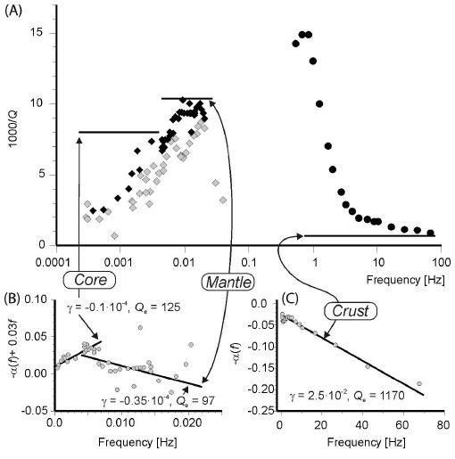
▲ Figure 1. (A) Observed 1000Q–1 for spherical oscillations, Rayleigh and P waves (gray diamonds), torsional oscillations, Love and S waves (black diamonds) from Anderson and Given (1982), and borehole S-wave data from Abercrombie (1998) (black circles). (B) and (C) The same S-wave data in –α(ƒ) form and in linear frequency scales for the (B) low-frequency and(C) high-frequency bands. In (B), a linear term 0.03ƒ was added to –α(ƒ) to make the trends near-horizontal and better resolved graphically. Note the three interpreted linear trends (solid lines), with γ and Qe values indicated
By way of conclusion, note that exploration seismologists often admit that their predictions are correct in only 25% of the cases, even though they take advantage of well-controlled experiments, vast amounts of data, and a lot more regular and shallower targets. This stark reality is established by drilling and competition, making it impossible to rely on conventions and underconstrained inversions. The domain of earthquake seismology is significantly more complex, and therefore its success rate does not have to be even that high. Verification of seismological interpretations may be subtle and difficult, and it requires periodic, unprejudiced reassessments of even classical models and conclusions in light of new ideas and data. Data should be the ultimate arbitrator, and their critical analysis should definitely be useful for both advancement of our knowledge and overcoming stereotypes. ![]()
REFERENCES
Abercrombie, R. E. (1998). A summary of attenuation measurements from borehole recordings of earthquakes: The 10 Hz transition problem. Pure and Applied Geophysics 153, 475–487.
Aki, K. (1980). Scattering and attenuation of shear waves in the lithosphere. Journal of Geophysical Research 85, 6,496–6,504.
Anderson, D. L., and J. W. Given (1982). Absorption band Q model for the Earth. Journal of Geophysical Research 87, 3,893–3,904.
Chernov, L. A. (1960). Wave Propagation in a Random Medium. New York: McGraw-Hill, 168 pps.
Morozov, I. (2008). Geometrical attenuation, frequency dependence of Q, and the absorption band problem. Geophysical Journal International 175, 239–252.
To send a letter to the editor regarding this opinion or to write your own
opinion, you may contact the SRL editor by sending e-mail to
<lastiz [at] ucsd [dot] edu>.
[Back]
Posted: 23 December 2008