|
|
Publications: SRL: EduQuakes |
EduQuakes
January/February 2012
QuakeCaster, an Earthquake Physics Demonstration and Exploration Tool
Kelsey Linton1 and Ross S. Stein2
 Authors' Affiliations") Click to Show (or Hide) Authors' Affiliations
Click to Show (or Hide) Authors' Affiliations
- Duke University, Durham, North Carolina, U.S.A.
- U.S. Geological Survey, Menlo Park, California, U.S.A.
INTRODUCTION
A fundamental riddle of earthquake occurrence is that tectonic motions at plate interiors are steady, changing only subtly over millions of years, but at plate boundary faults, the plates are stuck for hundreds of years and then suddenly jerk forward in earthquakes. Why does this happen? The answer, as formulated by Harry F. Reid (Reid 1910, 192) is that the Earth’s crust is elastic, behaving like a very stiff slab of rubber sliding over a substrate of “honey”-like asthenosphere, and that faults are restrained by friction. The crust near the faults—zones of weakness that separate the plates—slowly deforms, building up stress until frictional resistance on the fault is overcome and the fault suddenly slips. For the past century, scientists have sought ways to use this knowledge to forecast earthquakes.
QuakeCaster, a hands-on teaching model, simulates earthquakes and their interactions to help students explore and test the four leading hypotheses for earthquake occurrence. The model also allows students to extend these concepts to consider more complex earthquake interactions, clustering, and Coulomb stress triggering.
The four leading hypotheses for earthquake occurrence essentially trend from the most uniform and predictable behavior to the most irregular and unpredictable. Hypothesis 1 states that earthquakes are periodic: all have the same amount of slip, and all are separated by the same amount of time (Schwartz and Coppersmith 1984). In hypothesis 2, earthquakes are “time-predictable”: the larger the slip in the last earthquake, the longer the wait until the next one (Shimazaki and Nakata 1980). In hypothesis 3, earthquakes are “slip-predictable”: the longer the time since the last earthquake, the greater the size of the next earthquake (Bufe et al. 1977). In hypothesis 4, known as the “Poisson” hypothesis, earthquakes occur randomly in time and have randomly varying sizes (Campbell 1982). In the Poisson hypothesis, the next earthquake is not conditioned on or affected by the preceding earthquake.
QuakeCaster DESIGN AND PURPOSE
This model contains the minimum number of elements needed to reproduce most observable features of earthquake occurrence: a reel that steadily pulls in a line simulates the steady plate tectonic motions far from the plate boundaries, a granite slider in frictional contact with a porcelain surface simulates a plate boundary fault, and a rubber band connecting the line and the slider furnishes the elastic character of the earth’s crust (Figure 1). By stacking and unstacking sliders and steadily cranking the reel, one can see the effect of changing the shear and clamping (also called “normal”) stress on the fault. By placing sliders in series with rubber bands between them, one can simulate the interaction of several earthquakes along a fault, such as cascading (one earthquake leading to another) or toggling (one earthquake turning on when another turns off) shocks (Figure 2A). By inserting a load scale into the line, one can measure the Coulomb stress acting on the fault throughout the earthquake cycle (Figure 2B). With a stopwatch and ruler one can measure and plot the results (Figure 3A).
QuakeCaster is designed so that students or audience members can operate it themselves and can measure its output. We have used QuakeCaster with people of all ages and scientific backgrounds, from schoolchildren to seismologists. They are able to measure the time between events, slip distance (a stand-in for earthquake magnitude), and stress before and after an event occurs. Despite its simplicity, QuakeCaster exhibits remarkable fidelity to observed earthquake behavior. Students will get a memorable hands-on look at stress and rupture in the laboratory and will understand why it is so difficult to predict earthquakes in the real world. QuakeCaster costs $500–750 to build and takes several days to construct. For instructions on how to build QuakeCaster and a more comprehensive guide to teaching with it, see Linton and Stein (2011).

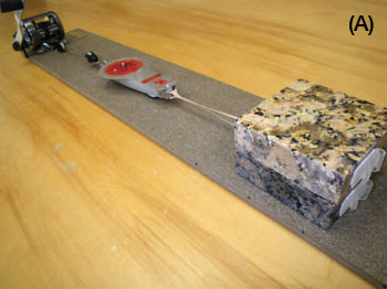
▲ Figure 1. Volkan Sevilgen marks the rupture length for each event while Kelsey Linton cranks the reel. A piece of white electrical tape has been placed along the edge of the porcelain tile. A force scale is used to measure the earthquake stress drop. The stopwatch on the table can be used to record the earthquake times.
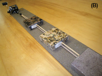
▲ Figure 2. (A) Three granite sliders in series, representing multiple earthquakes along a fault. Students make predictions about how sliders will interact through the transfer of stress. (B) Two stacked sliders with a stress gauge. Students make predictions about what stress earthquakes will occur at and what stress will drop to after an earthquake.
COULOMB FAILURE, STRESS TRIGGERING, AND EARTHQUAKE INTERACTION
QuakeCaster can demonstrate the Coulomb failure criteria, which hold that when a fault is close to failure, either increasing the shear stress (by reeling in a bit more line) or unclamping the fault (by lifting a stacked slider) will promote failure. To demonstrate increasing shear stress, stack two sliders and reel in the line until the slider is on the verge of slipping (Figure 2B). Now crank a bit more and it will trigger an earthquake. To demonstrate unclamping the fault, reel in the line again until the slider is on the verge of slipping, then lift the top slider. Again it will trigger a quake. If the static friction coefficient of the fault is about 0.5, then increasing the shear stress will have twice the impact of unclamping the fault in triggering an earthquake. The Coulomb hypothesis and the concept of earthquake stress triggering are explained in plain English in Stein (2003).
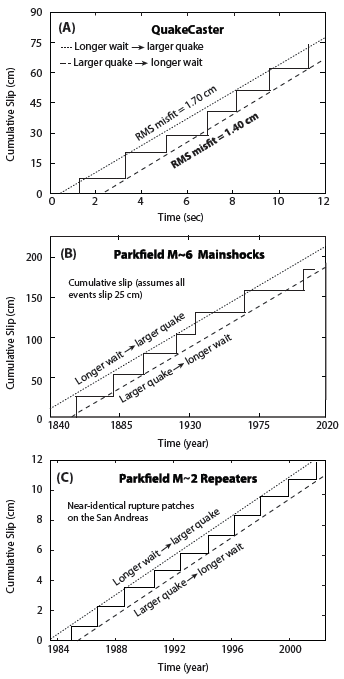
▲ Figure 3. Time- and slip-predictability in QuakeCaster and at Parkfield. (A) For QuakeCaster, the hypothesis in bold indicates better agreement with the observations for this trial. Here we used two stacked sliders. We did not count the time to the first earthquake because the spring starts fully unloaded. The M ~ 6 shocks (B) are neither time- nor slip-predictable, while the repeaters (C) are more periodic. The M ~ 6 data is from Bakun and McEvilly (1984) and Murray and Langbein (2006). Notice that the slip of QuakeCaster earthquakes is closer to the repeater slip than the repeaters are to the M ~ 6 shocks.
It is also possible for QuakeCaster to demonstrate how earthquakes converse with each other by the transfer of stress. Stress is defined as force divided by the surface area. Since the slider area is constant in QuakeCaster, we use force as a proxy (i.e., a substitute) for stress. One QuakeCaster experiment involves adding a second slider behind the first so that they are pulled in series. The sliders are joined by an elastic rubber band. When stress overcomes the frictional resistance on the fault, the first slider jumps forward, which increases the shear stress on the second slider. Eventually, perhaps after several earthquakes of the first slider, the second slider slips, and this reduces the restraining force on the first slider, and the first slider may slip again. We ask the audience to “wager” on which slider will rupture first, second, third, and fourth. They are almost always surprised by the outcome, which can change from one trial to the next, and the sliders’ interaction—sometimes exhibiting chaotic behavior—is much richer than one might expect. By making predictions of their own, students become invested in the outcome and more curious about earthquake behavior.
KEY QuakeCaster EXPERIMENTS
For our first experiment, we performed three trials to make “staircase” plots in which we measured the time between events and the slip distance. This required a minimum of three participants. We placed a piece of white tape along the side of the porcelain tile. Then, one person reeled at a constant rate (to simulate constant plate motion). A second person used a pen to mark on the tape the position of the slider after each earthquake to measure the slip. A third person held a lap-timer stopwatch and recorded the time of each event (one needs to measure in tenths of seconds).
After plotting the results (Figure 3A), one can see how the slip- and time-predictable hypotheses compare to the data by eyeballing and then drawing in the best-fitting lines to the staircase plots. For a more quantitative comparison of data to the models, one can calculate the root mean square (RMS) misfit value for the slip- and time- predictable hypotheses. (To calculate RMS misfit, subtract the predicted slip distance from the observed slip distance for each data point, square each result, add all the results together, divide this total amount by the number of data points, and take the square root.) At first glance, the earthquakes in this trial (Figure 3A) appear to fit the periodic hypothesis, but the RMS misfit values suggest differently. The misfit for the slip-predictable hypothesis is 1.7 cm, but for the time-predictable hypotheses it is 1.4 cm. Not all trials support the time- or slip-predictable hypotheses, and none of the trials perfectly match any of the four hypotheses.
These tests show how difficult it is to accurately predict earthquakes: even when we grossly oversimplify the likely complexity and variability in the earth, we still do not get regular, predictable earthquakes. This is perhaps the most important message of QuakeCaster.
One can quickly transcribe the observations to a PC and plot the QuakeCaster results, project them onto a whiteboard, and annotate them. Here’s how to plot them using Google Documents: (1) Open Google Documents and create a new spreadsheet. (2) Label one column “Time (sec)” and another column “Cumulative Slip (cm).” These will be the x- and y-axis labels. (3) Choose “insert chart” and select “scatter plot.” (4) Project the image onto a whiteboard. (5) Using a whiteboard pen and a straight edge, draw in a stair-step diagram to connect the dots. (6) Draw in eyeballed best-fit lines for slip- and time-predictability (or these could be done using the PC), and let people assess them. (7) For high school or college students, have them calculate the RMS misfit to the two hypotheses as we did in Figure 3.
Another valuable experiment is to test whether the failure stress is a more accurate predictor of earthquakes than their inter-event times and sizes. So, for our second experiment, we measured the force just before an earthquake occurred (the failure stress) and the force just after an earthquake occurred (the minimum or background stress) with the dial load scale. In order to ensure the most accurate data possible and to enhance involvement and interest, we used four people for this experiment. One person reeled, a second held the stopwatch and recorded the time of each event, a third recorded the force just before an event, and a fourth recorded the force just after an event. We performed three trials, and the results of one trial are shown in Figure 4A, together with laboratory data for Westerly granite (Lockner et al. 2011) that give comparable results (Figure 4B).
For each trial in the experiment on the failure stress and minimum stress, we calculated the RMS misfit to see if the data are better fit by a constant failure stress (equivalent to the time-predictable hypothesis) or a constant minimum or background stress (equivalent to slip-predictability). In this trial, the RMS misfit to the minimum stress is 80 grams, whereas to the failure stress it is 210 grams. In the three trials, there was no fixed failure stress. Surprisingly, the trials indicate that the minimum stress is a better predictor of earthquakes than the failure stress. As with the staircase plots, no trials perfectly fit either hypothesis. Equally important, notice that the stress never goes to zero: just as in actual earthquakes, the stress drop is much smaller than the total stress.
After running QuakeCaster just once (about four to six earthquakes), granite fault gouge is visible as a light dusting on the raised portions (or “asperities”) of the porcelain tile. Let people feel the gouge with their fingers. Gouge occurs in faults as a result of friction between fault faces when they slide past each other, and grind rocks into a pulverized powder. Moore and Rymer (2007) found saponite and talc in fault gouge within the San Andreas fault at the San Andreas Fault Observatory at Depth (SAFOD) drill site near Parkfield. These minerals decrease friction within faults and could therefore be responsible for fault creep at shallower (the saponite zone) and greater (the talc zone) depths along the San Andreas. Lockner et al. (2011) found that smectite clay also contributes to the San Andreas fault’s weakness at the SAFOD drilling site.
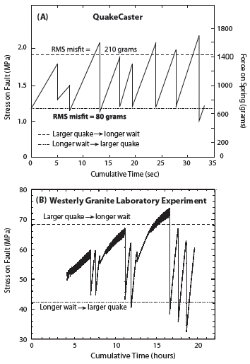
▲ Figure 4. Test trials of whether there is a constant minimum or failure stress. (A) QuakeCaster suggests that minimum stress might be a better earthquake predictor than failure stress. The hypothesis in bold indicates better agreement with the observations in this trial. Here we used two stacked sliders. (B) A 3-inch diameter cylinder of Westerly granite with a 30° saw-cut and 600-grit abrasive lapping of fault surfaces, sheared under constant confining pressure of 50 MPa and a constant loading rate of 0.1 micron/s (Lockner et al. 2011). Here, neither a constant failure stress nor a minimum stress forecasts the laboratory earthquakes. (For stress conversion, 1,000 KPa = 1 MPa = 10 bar.)
Using QuakeCaster, students can calculate the friction coefficient by dividing the force before an event by the weight of the slider(s). Or, slowly tilt the tile until the slider begins to move, and then measure the angle between the table and the tile; the tangent of the angle is the friction coefficient. Our tests have shown a friction coefficient around 0.5. However, the coefficient can change during the experiment. For example, if fault gouge accumulates over multiple trials, the coefficient tends to decrease. Since each slider has a polished upper surface, flipping it over will drop the friction to about 0.1–0.2. Try it: this produces more creep-like behavior in experiments and illustrates the profound importance of friction in earthquake occurrence.
HOW QuakeCaster STACKS UP AGAINST ACTUAL EARTHQUAKES
The Parkfield section of the San Andreas fault has hosted perhaps the most periodic earthquake sequence known on Earth, but it is neither time- nor slip-predictable (Figure 3B). At first glance, Parkfield appears to be roughly periodic, with magnitude 6 earthquakes every 20–30 years. However, the 1934 Parkfield earthquake occurred roughly a decade earlier than the average interval (Stein 2002; Scholz 2002, 473). Murray and Segall (2002) also concluded that the Parkfield magnitude 6 earthquakes are not time-predictable. Based on the 1850– 1966 inter-event times, the most recent earthquake after 1966 should have occurred sometime between 1973 and 1987, but it did not strike until 2004, about one to two decades late, and it was also somewhat larger than its recent predecessors. This record emphasizes that even the most predictable earthquakes deviate from the slip- or time-predictable hypotheses.
Even though the M ~ 6 Parkfield shocks are not periodic or time- and slip-predictable, there is a class of very small (M = 1−3) shocks, known as repeaters, whose seismic waveforms are nearly identical, and so are thought to occur at the same location and have the same size and slip (Figure 3C). At first glance, the set of M ~ 2 repeaters appears periodic, and it is certainly more periodic than the QuakeCaster shocks in Figure 3A and the M ~ 6 shocks in Figure 3B. But upon closer inspection, the repeaters are not periodic, nor are they time- or slip-predictable, as demonstrated by Rubenstein, Ellsworth, Chen et al. (forthcoming) and Rubenstein, Ellsworth, Beeler et al. (forthcoming).
The QuakeCaster stacked-slider earthquakes are M ~ −4.5. This means that the scale difference between the M ~ 6 and the repeating M ~ 2 events at Parkfield is about the same as the difference between the repeaters and QuakeCaster events. To estimate the QuakeCaster magnitude we calculated the seismic moment of a typical event from the slip (~10 cm), slider area (~100 cm²), rubber band cross-section (~0.1 cm² ), Poisson’s ratio (~0.25), and length change of the rubber band in response to a tensional load to calculate its Young’s modulus (~6 × 10⁶ dyne-cm−2). We converted Young’s modulus to the shear modulus, arriving at the seismic moment (~3 × 10^9 dyne-cm), which we then converted to magnitude.
Students can easily perform these calculations by measuring the change in length of the rubber band for a given force on the dial scale. Young’s modulus, E, is the tensile stress divided by tensile strain, which equals the force on the rubber band (F) multiplied by the original length of the rubber band (Lo) divided by the original cross-section of the rubber band (Ao) multiplied by the length change (ΔL); the full equation is FLo / AoΔL. Young’s modulus, E, can be converted to the shear modulus G, by G = E/2(1 + v). The seismic moment (Mo) is calculated by multiplying the slip (u), by the area of the fault (A), by the shear modulus (G). Finally, the magnitude, M, is 2/3(log Mo − 16.1).
CONCLUSIONS
We created QuakeCaster to enable student, scientific, and public audiences to develop an intuitive understanding of the Earth’s earthquake machine. We believe that QuakeCaster could serve as a valuable hands-on demonstration tool in college and university geology and seismology classes, and it would also help faculty and earthquake professionals communicate earthquake science to the public. It is inexpensive to build and can be checked as airline baggage, so it is both affordable and transportable. But at four feet long, it is large and noisy enough that an audience of 100 people can easily see and hear what is happening. To see and hear it in action, we have created a three-minute trailer (http://www.youtube.com/watch?v=zIipwGUaFAk&feature=player_embedded) and an 11-minute “How to Teach with QuakeCaster” video (http://www.youtube.com/watch?v=Y3Xt3qgV63c&feature=player_embedded); they can also be accessed through Linton and Stein (2011).
We have found QuakeCaster speaks to middle school students, graduate students, the public, insurance executives, and research seismologists. It illuminates Earth processes and encourages experimentation while making learning fun. People are vocal and eager to share their observations, traits that are crucial to scientific inquiry and discovery. By involving audience members in experiments, QuakeCaster makes it easy to see why it is so difficult to predict earthquakes.
ACKNOWLEDGMENTS
We thank Volkan Sevilgen, Jacob DeAngelo, Brian Kilgore, Benjamin Hankin, and Patty McCrory for advice, innovations, and assistance while we designed, prototyped, and tested QuakeCaster. We thank David Lockner, Diane Moore, Alan Kafka, and Menlo Middle School science teacher Tammy Cook for perceptive reviews. We are also grateful to Jacob for coming up with its name!
REFERENCES
Bakun, W. H., and T. V. McEvilly (1984). Recurrence models and Parkfield, California, earthquakes. Journal of Geophysical Research 89, 3,051–3,058.
Bufe, C. G., P. W. Harsh, and R. O. Burford (1977). Steady-state seismic slip—a precise recurrence model. Geophysical Research Letters 4, 91–94; doi:10.1029/GL004i002p00091.
Campbell, K. W. (1982). Bayesian analysis of extreme earthquake occurrences. Part I. Probabilistic hazard model. Bulletin of the Seismological Society of America 72, 1,689–1,705.
Linton, K., and R. S. Stein (2011). How to Build and Teach with QuakeCaster, an Earthquake Demonstration and Exploration Tool. USGS Open-File Report 2011-1158, 34 pp. See http://pubs.usgs.gov/of/2011/1158.
Lockner, D. A., C. Morrow, D. Moore, and S. H. Hickman (2011). Low strength of deep San Andreas fault gouge from SAFOD core. Nature 472, 82–85.
Moore, D. E., and M. J. Rymer (2007). Talc-bearing serpentinite and the creeping section of the San Andreas fault. Nature 448, 795–797.
Murray, J., and J. Langbein (2006). Slip on the San Andreas fault at Parkfield, California, over two earthquake cycles, and the implications for seismic hazards. Bulletin of the Seismological Society of America 96, S283–S303; doi:10.1785/0120050820.
Murray, J., and P. Segall (2002). Testing time-predictable earthquake recurrence by direct measure of strain accumulation and release. Nature 419, 287–291.
Reid, H. F. (1910). The mechanics of the earthquake. In The California Earthquake of April 18, 1906. Report of the State Earthquake Investigation Commission, vol. 2, ed. A. C. Lawson,
Rubinstein, J. L., W. L. Ellsworth, N. Beeler, B. D. Kilgore, D. Lockner, and H. Savage (forthcoming). Fixed recurrence and slip models better predict earthquake behavior than the time- and slip-predictable models 2: Laboratory earthquakes. Journal of Geophysical Research.
Rubinstein, J. L., W. L. Ellsworth, K. H. Chen, and N. Uchida (forthcoming). Fixed recurrence and slip models better predict earthquake behavior than the time- and slip- predictable models 1: Repeating earthquakes. Journal of Geophysical Research.
Scholz, C. H. (2002). The Mechanics of Earthquakes and Faulting. 2nd ed. Cambridge: Cambridge University Press, 473. Schwartz, D. P., and K. J. Coppersmith (1984). Fault behavior and characteristic earthquakes: Examples from the Wasatch and San Andreas fault zones. Journal of Geophysical Research 89, 5,681– 5,698; doi:10.1029/JB089iB07p05681.
Shimazaki, K., and T. Nakata (1980). Time-predictable recurrence model for large earthquakes. Geophysical Research Letters 7, 279–282.
Stein, R. S. (2002). Parkfield’s unfulfilled promise. Nature 419, 257–258.
Stein, R. S. (2003). Earthquake conversations. Scientific American 288, 72–79.
[ Back ]
| HOME |
Posted: 20 December 2011