|
|
Publications: SRL: EduQuakes |
EduQuakes
March/April 2012
Listening to the 2011 Magnitude 9.0 Tohoku-Oki, Japan, Earthquake
Zhigang Peng,1 Chastity Aiken,1 Debi Kilb,2 David R. Shelly,3 and Bogdan Enescu4
 Authors' Affiliations") Click to Show (or Hide) Authors' Affiliations
Click to Show (or Hide) Authors' Affiliations
- School of Earth and Atmospheric Sciences, Georgia Institute of Technology, Atlanta, Georgia, U.S.A.
- Institute of Geophysics and Planetary Physics, University of California, San Diego, La Jolla, California, U.S.A.
- Volcano Science Center, U.S. Geological Survey, Menlo Park, California, U.S.A.
- National Research Institute for Earth Science and Disaster (NIED), Tsukuba, Japan
Online Material: Six supplemental movies
INTRODUCTION
The magnitude 9.0 Tohoku-Oki, Japan, earthquake on 11 March 2011 is the largest earthquake to date in Japan’s modern history and is ranked as the fourth largest earthquake in the world since 1900. This earthquake occurred within the northeast Japan subduction zone (Figure 1), where the Pacific plate is subducting beneath the Okhotsk plate at rate of ~8–9 cm/yr (DeMets et al. 2010). This type of extremely large earthquake within a subduction zone is generally termed a “megathrust” earthquake. Strong shaking from this magnitude 9 earthquake engulfed the entire Japanese Islands, reaching a maximum acceleration ~3 times that of gravity (3 g). Two days prior to the main event, a foreshock sequence occurred, including one earthquake of magnitude 7.2. Following the main event, numerous aftershocks occurred around the main slip region; the largest of these was magnitude 7.9. The entire foreshocks-mainshock-aftershocks sequence was well recorded by thousands of sensitive seismometers and geodetic instruments across Japan, resulting in the best-recorded megathrust earthquake in history. This devastating earthquake resulted in significant damage and high death tolls caused primarily by the associated large tsunami. This tsunami reached heights of more than 30 m, and inundation propagated inland more than 5 km from the Pacific coast, which also caused a nuclear crisis that is still affecting people’s lives in certain regions of Japan.
As seismologists, it is important that we effectively convey information about catastrophic earthquakes, like this recent Japan event, to others who may not necessarily be well versed in the language and methods of earthquake seismology. Until recently, it was typical to only use “snapshot” static images to represent earthquake data. From these static images alone it was often difficult to explain even the basic characteristics of seismic waves generated by earthquakes, such as primary (P), secondary (S), and surface waves. More advanced aspects of the seismic waves, such as frequency content, attenuation, site effects, and phenomena such as earthquake triggering were even more difficult to explain. This was especially true for general audiences, such as high school students, who do not have prior knowledge of basic seismology. Recently, animations and visualizations have been increasingly used to present information about earthquakes and how seismic waves propagate inside the Earth (e.g., http://www.iris.edu/hq/programs/education_and_outreach/ visualizations). However, most of these animations do not take advantage of people’s ability to learn through sound cues such as amplitude, pitch, and frequency. Here, we take an alternative approach and convert seismic data into sounds, a concept known as “audification” or continuous “sonification” (e.g., Walker and Nees 2011).
By combining seismic auditory and visual information, static “snapshots” of earthquake data come to life, allowing the viewer to hear pitch and amplitude changes in sync with viewed frequency changes in the earthquake seismograms. In addition, this approach allows the audience to relate seismic signals generated by earthquakes to familiar sounds such as thunder, popcorn popping, rattlesnakes, gunshots, firecrackers, etc. Thus, audification of seismic data can be an effective tool to convey useful information about earthquake recordings, seismic wave propagation inside the Earth, and interaction of seismic events with one another.
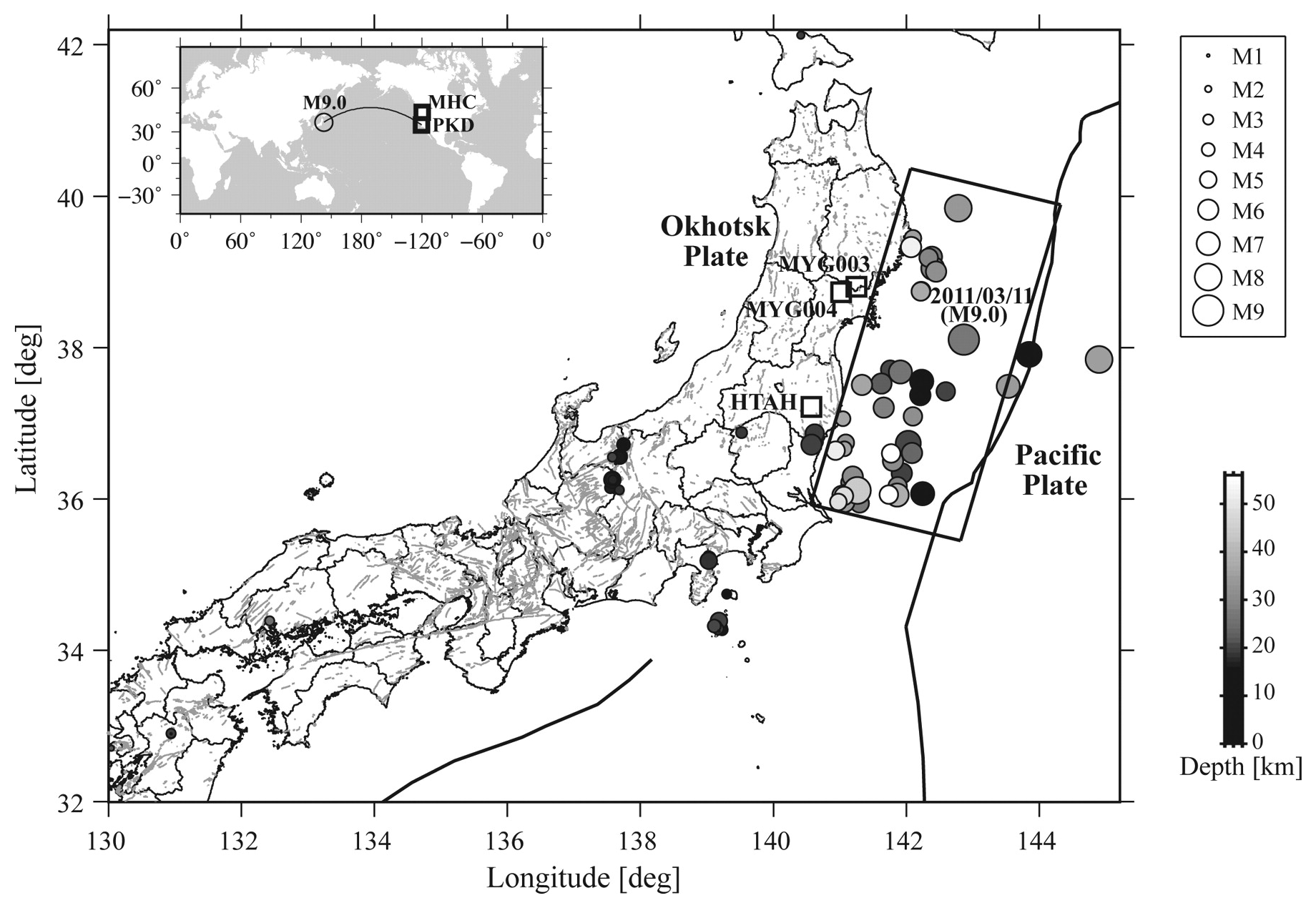
▲ Figure 1. Map showing Japanese seismicity, as recorded in the JMA catalog, in the first hour from the Tohoku-Oki mainshock. The earthquakes are shown as circles with sizes that scale with their magnitudes and colored (gray-scale) according to their depth location. The K-net stations MYG003 and MYG004 and the Hi-net station HTAH, which are used in this paper, are marked as small rectangles. The large black rectangle represents the fault area (Suzuki et al. 2011) of the 2011 Tohoku-Oki earthquake, projected on the surface. The faults in inland Japan are shown as thick gray lines and the trenches are shown as thick black lines. For the online supplementary movie 1 we use the occurrence times of earthquakes with epicenters within or close to the fault region. The inset shows the global map with the ray path between the mainshock and station PKD around the Parkfield section of the San Andreas fault in central California. Station MHC in northern California is also marked.
The concept of audification in seismology has existed for several decades (Benioff 1953; Speeth 1961; Hayward 1994; Dombois and Eckel 2011) and was recently brought up in several conference proceedings (Simpson 2005; Simpson et al. 2009; Fisher et al. 2010). The audible frequency range for human hearing is roughly 20 Hz–20 kHz, which is on the high end of the frequency range for earthquake signals recorded by modern seismometers (~100 s or 0.01 Hz –~100 Hz). The easiest way to make seismic data audible is to play it much faster than true speed, also known as time-compression or speed-up (e.g., Hayward 1994; Dombois and Eckel 2011). Doing so allows a direct mapping of the seismic frequency range into the audible frequency range. In addition, with time compression it takes much less time to play the resulting sound track, so the audience can hear seismic signals that typically occur over a few hours in a matter of about a minute. In a companion paper, Kilb et al. (2012, this issue’s Electronic Seismologist column) demonstrate how to convert seismic data into sounds and movies using simple tools such as MATLAB and Apple Inc.’s QuickTime Pro. Here we show a few examples generated by those tools using data from in the north-south direction at station MYG004. In addition the 2011 Tohoku-Oki earthquake to help convey important to showing the original data, we apply a 20-Hz high-pass filinformation about the Japan earthquake to general audiences.
EXAMPLE 1: NEAR-FIELD STRONG GROUND-MOTION RECORDING OF THE MAINSHOCK
The Mw 9.0 Tohoku-Oki, Japan, earthquake was recorded by two of the world’s densest strong-motion seismic networks, namely the K-net and the KiK-net. The K-net consists of more than 1,000 strong-motion seismographs at the ground surface, while the KiK-net consists of ~700 stations with a surface/ downhole pair of strong-motion seismographs (Okada et al. 2004). Both networks recorded the mainshock ground accelerations, and the highest acceleration of nearly 3 g was recorded at one K-net station (station code MYG004) near the mainshock epicenter. In this example we use ground acceleration in the north-south direction at station MYG004. In addition to showing the original data, we apply a 20-Hz high-pass filter to remove the low-frequency content in order to show the high-frequency signals in the data (Peng et al. 2007). We also include a spectrogram, which is a colorful image to show how the spectral content of a signal varies with time. Generally the horizontal axis in a spectrogram plot represents time and the vertical axis is frequency, and intensity or color of each point corresponds to the amplitude or energy of a certain frequency at a particular time.
As shown in Figure 2, the recorded data mainly consist of two groups of ground motion. It takes ~50 seconds for the seismic data to reach initial peak amplitude. After that, there is a brief amplitude decrease, and then at ~90 seconds, the second and the highest peak amplitude is reached. These strong high-frequency signals end at around 180 s. This double-peaked signature in ground motion amplitudes is also observed at many nearby seismic stations, suggesting at least two patches of high-frequency radiation from the mainshock rupture (Ide et al. 2011; Suzuki et al. 2011).
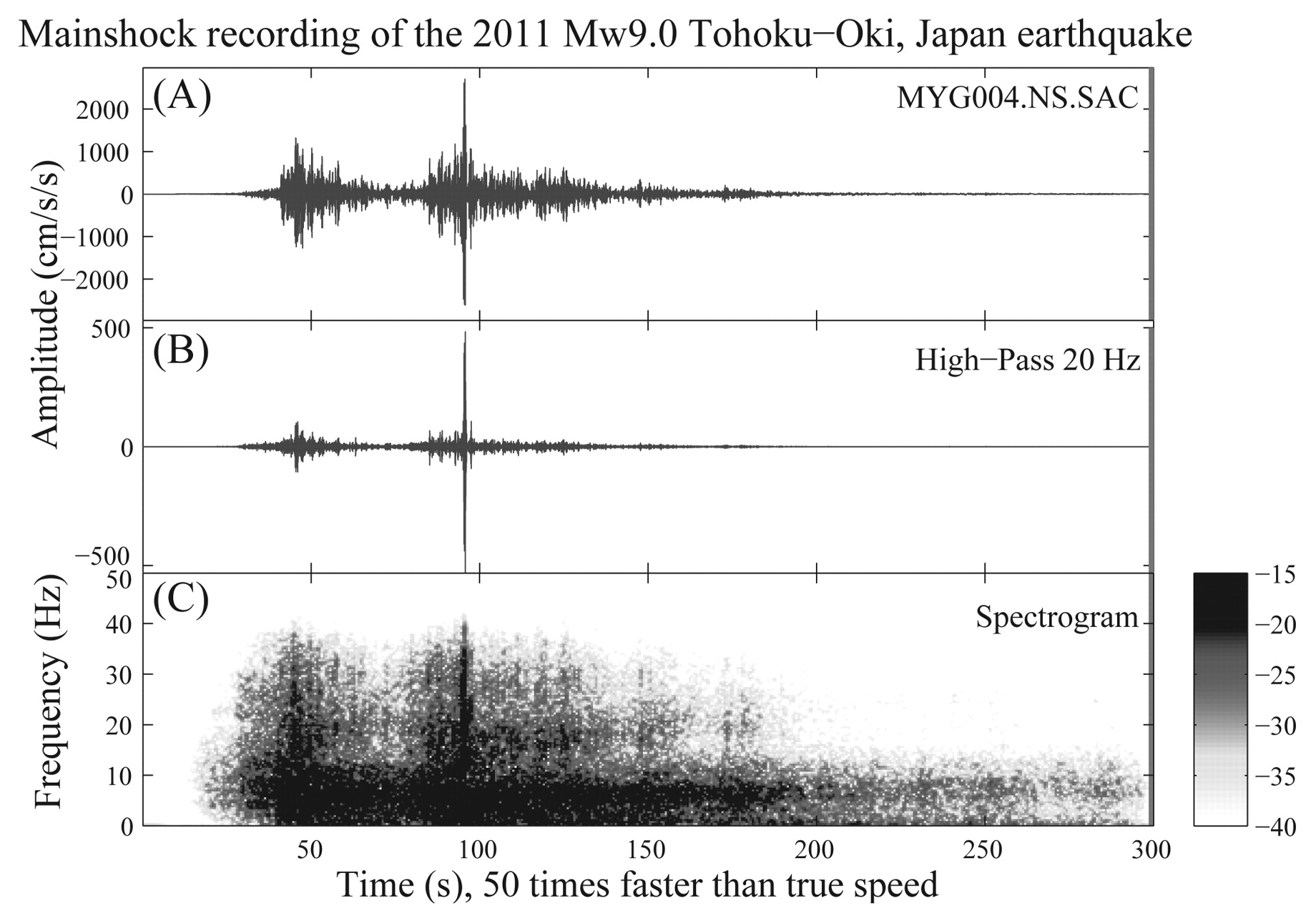
▲ Figure 2. Example of near-field strong-motion recordings at K-Net station MYG004 during the 2011 Mw 9.0 Tohoku-Oki earthquake. (A) North-component acceleration seismogram. (B) 20-Hz high-pass-filtered seismogram. (C) The spectrogram of the north-component seismogram. The signal associated with the highest ground acceleration at ~ 90 s has higher frequency content than those at other times. A 0.5-Hz high-pass filter is applied before computing the spectrogram in order to reduce the high-frequency artifact generated from applying a short-time-window Fourier transform to a long-period signal (Peng, Long, and Zhao 2011). The corresponding movie with color and sound is shown in the online supplementary movie 1.
The corresponding sound and video of the N-S component data (speeded up by a factor of 50) is shown in the online supplementary movie 1. From the sound component of this movie we can hear two groups of loud noises, consistent with what is shown in the static image (Figure 2). We note that the highest ground acceleration occurred ~90 s after the mainshock rupture began. The frequency content during this time period is much higher, and the corresponding sound has much higher pitch as compared with other times. For comparison, we show the animation of the N-S component recorded at a nearby station MYG003 (online supplementary movie 2). Because the ultra high-frequency signal at ~90 s was not recorded at station MYG003 and other nearby stations, we hypothesize that such high-frequency radiation might be generated by a very shallow seismic event immediately beneath station MYG004 (Fischer et al. 2008; Sleep and Ma 2008). Alternatively, this could be caused by local site effects or topographic amplifications (Skarlatoudis and Papazachos 2012). We plan to investigate this further in a follow-up study. The purpose of this example is to demonstrate variable strong ground motions produced by the mainshock.
EXAMPLE 2: EARLY AFTERSHOCKS OF THE TOHOKU-OKI, JAPAN, EARTHQUAKE
Large shallow earthquakes are typically followed by a significant increase in seismic activity near the mainshock rupture that is generally termed “aftershock.” The Tohoku-Oki earthquake triggered numerous aftershocks that were recorded on scale by many nearby instruments. Figure 3 shows the seismic data recorded on the vertical component of the Hi-net borehole station HTAH starting 100 s before and ending one hour after the occurrence time of the mainshock. Hi-net is a high-sensitivity seismograph network that records velocity motions with ~800 stations mostly placed in the same boreholes as the KiK-net stations at a typical depth of 100 to 200 m (Okada et al. 2004). The raw seismic data clearly show the mainshock and some large aftershock signals (Figure 3A). In addition, we apply a 20-Hz high-pass filter to remove low-frequency content and compute an envelope function, which is a curve that captures the overall shape of the signal. We finally take base-10 logarithm to show both strong and weak signals. The resulting envelope function (Figure 3B) and the spectrogram (Figure 3C) clearly mark many high-frequency bursts, which are primarily generated by aftershocks immediately following the Tohoku-Oki mainshock.
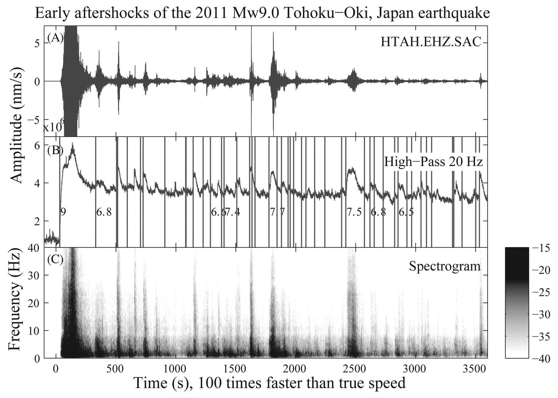
▲ Figure 3. Example of the mainshock and early aftershock recordings during the 2011 Mw 9.0 Tohoku-Oki earthquake. (A) Vertical-component velocity seismogram recorded at the Hi-net station HTAH. (B) 20-Hz highpass-filtered envelope functions highlighting the mainshock and early aftershock signals. The envelope function is smoothed with a half width of 50 data points and is in base 10 logarithmic scale. The black lines mark the predicted P-wave arrivals of aftershocks around the mainshock slip region as listed in the JMA earthquake catalog. (C) The spectrogram. The corresponding movie with color and sound is shown in the online supplementary movie 3.
In the corresponding sound and video (online supplementary movie 3), the aftershock signals sound like a rapid-fire gunshot or “pop-it” firecrackers that have been thrown on the ground. In this case, we speed up the seismic data 100 times to reduce the playback time. The resulting sound contains higher pitch than in the previous examples when it was speeded up only 50 times. In addition, we also set the maximum amplitude to be 1/50 of the peak mainshock value so that the weak aftershock sounds can be better heard. In this case, the mainshock signal is clipped or distorted so the resulting sound is noisier. We also mark with a black line the occurrence time of each aftershock around the mainshock rupture region (Figure 1) listed in the Japan Meteorological Agency (JMA) earthquake catalog. From the absence of an aftershock marker for some vertical peaks (i.e., aftershocks) in the envelope function it is evident that some aftershocks are not listed in the catalog. A systematic analysis of those missing aftershocks is currently underway (Lengliné et al. 2011) for better understanding the transition from mainshock to aftershocks and the physical mechanisms that control aftershock generation around the mainshock slip region (Enescu et al. 2007; Kilb et al. 2007; Peng et al. 2007).
EXAMPLE 3: REMOTE TRIGGERING OF TREMOR IN CENTRAL CALIFORNIA
Recent studies have shown that large earthquakes could trigger or cause additional small earthquakes and deep tremor activities at several hundred to thousands of kilometers away (e.g., Peng and Gomberg 2010). Similarly, the Tohoku-Oki mainshock also triggered numerous earthquakes and tremor around the world (Peng et al. 2011). The major difference between tremor and earthquake signals is that tremor occurs at greater depths and ruptures with slower speed than regular earthquakes (Peng and Gomberg 2010). Hence a tremor’s frequency content is lower, and the corresponding sound has lower pitch, than that of a regular earthquake. In addition, tremor often occurs in groups and hence sounds less distinct than earthquake swarms or aftershocks. Here we show two examples of triggered tremor activities recorded by the broadband station PKD along the Parkfield-Cholame section of the San Andreas fault in central California, which are ~8,000 kilometers away from the mainshock event.

▲ Figure 4. Example of triggered tremor around the Parkfield-Cholame section of the San Andreas fault during the teleseismic waves of the 2011 Mw 9.0 Tohoku-Oki earthquake. (A) Broadband transverse-component seismogram recorded at station PKD. The two vertical lines mark the approximate arrival times of the P and S waves. (B) 2–16 Hz bandpass-filtered transverse-component seismogram showing the teleseismic P waves and locally triggered tremor signals during the teleseismic S and surface waves. (C) Spectrogram of the transverse-component seismogram recorded at station PKD. The triggered tremor signals can be identified by the narrow vertical bands indicating richness in high-frequency energy. The corresponding movie with color and sound is shown in the online supplementary movie 4.
Seismic data recorded at station PKD, which is part of the Berkeley Digital Seismic Network (BDSN), contains both the long-period signals of the distant Japan earthquake and high-frequency triggered tremor signals that occurred locally beneath the San Andreas fault (Figure 4). The tremor signals began right at the time when the S wave from the Japan earthquake arrived at Parkfield and became further intensified and modulated by the long-period surface waves. The associated sound and video (online supplementary movie 4) contains a loud low-pitch noise (like thunder) corresponding to the arrival of the mainshock P wave, followed by a high-pitch sound (like rainfall) that turns on and off frequently and corresponds well with the long-period seismic signals from the distant event. The latter is associated with the deep tremor signals that were triggered/modulated by the S wave and surface wave signals (Peng et al. 2009). For comparison, online supplementary movie 5 presents the sound and video generated from data at another broadband station MHC ~180 km north near the Calaveras fault in northern California. It contains the same thunder-like P-wave sound at the beginning, but without the follow-up rainfall-like tremor sound during the S and surface waves. Two local earthquakes with sounds similar to gunshots occurred at ~2,900 s after the mainshock origin time. Such a comparison clearly demonstrates that the high-pitch sound at station PKD during the S and surface waves is unusual and likely produced by local fault movement triggered by the distant earthquake.
In the next example, we include a cross-sectional map of the tremor locations (Shelly and Hardebeck 2010) along the San Andreas fault, together with the seismic waveform data (Figure 5 and online supplementary movie 6). In this case, the location of each tremor “lights up” as a deep red circle when it first occurs and then fades in color and shrinks in size to help the viewer track possible migration of tremor activity (Shelly 2010; Shelly et al. 2011). This visualization shows that the tremor during the mainshock S wave first occurred in the NW direction around the creeping section of the San Andreas fault. Most of the tremor, however, occurred around Cholame, in the SE direction, during the subsequent surface waves. Both this and previous examples clearly demonstrate how distant earth-quakes like the Tohoku-Oki event can trigger deep fault movement thousands of kilometers away.

▲ Figure 5. Example of triggered tremorduring the 2011 Mw 9.0 Tohoku-Oki earthquake. (A) A cross-section view along and parallel to the Parkfield-Cholame section of the San Andreas fault. The small dots mark the hypocenters of regular earthquakes, and the small black “plus” symbols show tremor family source locations. (B) A velocity seismogram recorded near Parkfield, filtered 4–9 Hz, showing mostly local energy. (C) Unfiltered velocity seismograms recorded by the broadband station PAGB: vertical component (upper plot) and transverse component (lower plot), showing mostly energy from the distant earthquake. The corresponding movie with color and sound is shown in the online supplementary movie 6.
SUMMARY AND FUTURE DIRECTIONS
Additional images, sounds, and videos created from the seismic data generated by the 2011 Tohoku-Oki mainshock can be found online at http://geophysics.eas.gatech.edu/people/zpeng/ Japan_20110311/. This allows anyone to access the data products freely. In addition, the Web site contains a link to download a MATLAB script “sac2wav.m” that can convert seismic data in the Seismic Analysis Code (SAC) format into the WAVE format. This open-source code provides those interested a chance to play with the data and create their own sound files. The detailed procedures to create the full video/sound files are described in the companion paper to this work (see Kilb et al. 2012, this issue’s Electronic Seismologist column).
The Web site was initially created on 6 April 2011 and has been modified several times since then. It was first presented at an online seminar series called “Teaching Geophysics in the 21st Century: Visualizing Seismic Waves for Teaching and Research” (http://serc.carleton.edu/ NAGTWorkshops/geophysics/seismic11/index.html), and later at the Seismological Society of America 2011 annual meeting. A link to this Web site has been included in several Education and Outreach (E&O) Web sites such as the Incorporated Research Institutions for Seismology (IRIS)’s special event Web site (http://www.iris.edu/news/events/japan2011/), allowing it to be reached by a wide audience.
The examples we present here and on our Web site are mostly used to demonstrate how the Tohoku-Oki mainshock triggered additional seismic events in the immediate vicinity (as aftershocks) and at large distances (such as tremor in Parkfield, CA). In these examples sound (pitch and amplitude) is related to the frequency spectrum and amplitude of seismograms, although depending on the research goals additional mapping could be defined. For example, the sound could be mapped to earthquake depths, mainshock/aftershock back-azimuths, or aftershock magnitudes (see for example http://pods.binghamton.edu/~ajones/#Seismic-Eruptions).In addition, similar products can be generated to illustrate how seismic waves propagate inside the Earth, and how different sites (solid rocks versus soft soils) could affect the amplitude and frequency content of the surface shaking (Michael 1997). We envision that audification of seismic data could be increasingly used to convey information to general audiences about recent earthquakes and research frontiers in earthquake seismology (tremor, dynamic triggering, etc.). Furthermore, we hope that sharing a new visualization tool will foster an interest in seismology not just for young scientists but also for people of all ages.
ACKNOWLEDGMENTS
Seismic data used in this study are downloaded from the Northern California Earthquake Data Center (NCEDC) and the National Research Institute for Earth Science and Disaster Prevention (NIED) Data Center in Japan. We thank the Japan Meteorological Agency (JMA) for its earthquake catalog. This manuscript benefitted from useful comments by Alan Kafka and Andrew Michael. This project is supported by the National Science Foundation (NSF) CAREER program EAR-0956051 to ZP and CA, and the IRIS sub-award 86-DMS funding 2011-3366 (DK). Any use of product, firm, or trade names is for descriptive purposes only and does not imply endorsement by the U.S. Government. Any use of product, firm, or trade names is for descriptive purposes only and does not imply endorsement by the U.S. Government.
REFERENCES
Benioff, H. (1953). Earthquakes around the world. On Out of This World, ed. E. Cook., side 2. Stamford, CT: Cook Laboratories, 5012 (LP record audio recording).
DeMets, C., R. G. Gordon, and D. F. Argus (2010). Geologically current plate motions. Geophysical Journal International 181, 1–80; doi:j.1365-246X.2009.04491.x.
Dombois, F., and G. Eckel (2011). Audification. In The Sonification Handbook, ed. T. Hermann, A. Hunt, and J. Neuhoff, 301–324. Berlin: Logos Publishing House http://sonification.de/handbook/index.php/chapters/chapter12/.
Enescu, B., J. Mori, and M. Miyazawa (2007). Quantifying early aftershock activity of the 2004 mid-Niigata Prefecture earthquake (Mw 6.6). Journal of Geophysical Research 112, B04310; doi:10.1029/2006JB004629.
Fischer, A., Z. Peng, and C. Sammis (2008). Dynamic triggering of high-frequency bursts by strong motions during the 2004 Parkfield earthquake sequence. Geophysical Research Letters 35, L12305; doi:10.1029/2008GL033905.
Fisher, M., Z. Peng, D. W. Simpson, and D. L. Kilb (2010). Hear it, see it, explore it: Visualizations and sonifications of seismic signals. Eos, Transactions, American Geophysical Union 91, Fall Meeting Supplement, Abstract ED41C-0654.
Hayward, C. (1994). Listening to the Earth sing. In Auditory Display: Sonification, Audification, and Auditory Interfaces, ed. G. Kramer, 369–404. Reading, MA: Addison-Wesley.
Ide, S., A. Baltay, and G. C. Beroza (2011). Shallow dynamic overshoot and energetic deep rupture in the 2011 Mw 9.0 Tohoku-Oki earth quake. Science 332, 1,426–1,429; doi:10.1126/science.1207020.
Kilb, D., V. G. Martynov, and F. L. Vernon (2007). Aftershock detection thresholds as a function of time: Results from the ANZA seismic network following the 31 October 2001 ML 5.1 Anza, California, earthquake. Bulletin of the Seismological Society of America 97 (3), 780–792; doi:10.1785/0120060116.
Kilb, D., Z. Peng, D. Simpson, A. Michael, and M. Fisher (2012). Listen, watch, learn: SeisSound video products. Seismological Research Letters 83, 281–286.
Lengliné, O., B. Enescu, Z. Peng, and K. Shiomi (2011). Unraveling the detailed aftershock sequence of the Mw = 9.0 2011 Tohoku mega-thrust earthquake through the application of matched filter tech niques. Abstract S13A-2252 presented at the 2011 Fall Meeting, America Geophysical Union, San Francisco, CA, December 5–9.
Michael, A. J. (1997). Listening to earthquakes. USGS; http://earthquake.usgs.gov/learn/listen/index.php.
Okada, Y., K. Kasahara, S. Hori, K. Obara, S. Sekiguchi, H. Fujiwara, and A. Yamamoto (2004). Recent progress of seismic observation networks in Japan—Hi-net, F-net, K-NET and KiK-net. Earth Planets Space 56, xv–xxviii.
Peng, Z., K. Chao, C. Aiken, D. R. Shelly, D. P. Hill, C. Wu, B. Enescu, and A. Doran (2011). Remote triggering following the 2011 M 9.0 Tohoku, Japan earthquake. Seismological Research Letters 82, 461 (abstract).
Peng, Z., and J. Gomberg (2010). An integrated perspective of the continuum between earthquakes and slow-slip phenomena. Nature Geoscience 3, 599–607; doi:10.1038/ngeo940.
Peng, Z., L. T. Long, and P. Zhao (2011). The relevance of high-frequency analysis artifacts to remote triggering. Seismological Research Letters 82 (5), 654–660; doi:10.1785/gssrl.83.2.654.
Peng, Z., J. E. Vidale, M. Ishii, and A. Helmstetter (2007). Seismicity rate immediately before and after main shock rupture from high-frequency waveforms in Japan. Journal of Geophysical Research 112, B03306; doi:10.1029/2006JB004386.
Peng, Z., J. E. Vidale, A. Wech, R. M. Nadeau, and K. C. Creager (2009). Remote triggering of tremor along the San Andreas fault in cen tral California. Journal of Geophysical Research 114, B00A06; doi:10.1029/2008JB006049.
Shelly, D. (2010). Migrating tremors illuminate deformation beneath the seismogenic San Andreas fault. Nature 463, 648–652; doi:10.1038/nature0875.
Shelly, D., and J. Hardebeck (2010). Precise tremor source locations and amplitude variations along the lower-crustal central San Andreas fault. Geophysical Research Letters 37, L14301; doi:10.1029/2010GL043672.
Shelly, D., Z. Peng, D. Hill, and C. Aiken (2011). Triggered creep as a possible mechanism for delayed dynamic triggering of tremor and earthquakes. Nature Geoscience 4, 384–388; doi:10.1038/NGEO1141.
Simpson, D. W. (2005). Sonification of GSN data: Audio probing of the Earth. Seismological Research Letters 76 (2), 263 (abstract).
Simpson, D. W., Z. Peng, D. Kilb, and D. Rohrick (2009). Sonification of earthquake data: From wiggles to pops, booms and rumbles. Abstract D53E-08 presented at the 2009 Fall Meeting, American Geophysical Union, San Francisco, CA, December 14–18 (abstract).
Skarlatoudis A. A. and C. B. Papazachos (2011). Preliminary Study of Ground Motions of Tohoku, Japan, Earthquake of 11 March 2011: Assessing the Influence of Anelastic Attenuation and Rupture Directivity. Seismological Research Letters 83, 119–129.
Sleep, N., and S. Ma (2008). Production of brief extreme ground acceleration pulses by nonlinear mechanisms in the shallow subsurface. Geochemistry, Geophysics, Geosystems 9, Q03008; doi:10.1029/2007GC001863.
Speeth, S. D. (1961). Seismometer sounds. Journal of the Acoustical Society of America 33, 909–916.
Suzuki, W., S. Aoi, H. Sekiguchi, and T. Kunugi (2011). Rupture process of the 2011 Tohoku-Oki mega-thrust earthquake (M 9.0) inverted from strong-motion data. Geophysical Research Letters 38, L00G16; doi:10.1029/2011GL049136.
Walker, B. N., and M. A. Nees (2011). Theory of sonification. In The Sonification Handbook, ed. T. Hermann, A. Hunt, and J. Neuhoff, 9–39. Berlin, Germany: Logos Publishing House.
[ Back ]
| HOME |
Posted: 28 February 2012