
FuncLab: A MATLAB Interactive Toolbox for Handling Receiver Function Datasets
Kevin C. Eagar 1,2 and Matthew J. Fouch 1,3
- Arizona State University, School of Earth and Space Exploration, Tempe, Arizona, U.S.A.
- Now at Shell Exploration and Production Company, Houston, Texas
- Now at Dept. of Terrestrial Magnetism, Carnegie Institution of Washington, Washington, DC
INTRODUCTION
Receiver functions have become a widely used tool to study the seismic velocity structure beneath a single station by imaging impedance boundaries where mode conversions from P to S waves occur. In recent years, the community has seen an increase in the amount of broadband seismic data available through systems such as the IRIS Data Management Center (IRIS DMC), requiring new approaches to managing and handling large datasets in computationally efficient ways. Many receiver function studies have focused on tectonic and geodynamic questions on regional scales of a few hundred square kilometers (e.g., Zandt et al. 1995; Sheehan et al. 1995; Dueker and Sheehan 1997). These studies typically have utilized data from temporary networks operating on time scales of a few months to a few years. Others have concentrated on global trends, using data from increasing numbers stations that have operated for years or decades (e.g., Andrews and Deuss 2008; Lawrence and Shearer 2006; Tauzin et al. 2008). Over the last several years, the seismological community has seen a rapid increase in the number of deployed passive broadband seismic stations and a resulting increase in data available for receiver function analysis. Large initiatives such as EarthScope’s USArray Transportable Array enable immediate open access to data and have provided the community with an order of magnitude more data than in the previous three decades (Figure 1) based on smaller regional temporary studies using data from IRIS PASSCAL-style field experiments (e.g., Suckale et al. 2009; Wilson et al. 2005).
While the computation of receiver functions has been well studied and is a relatively straightforward and rapid process, an efficient method to analyze and further evaluate very large receiver function datasets is not widely available. In this paper, we present an efficient workflow and MATLAB toolbox for organizing receiver function data, which we call FuncLab. FuncLab is a package of m-files (MATLAB scripts) written for the purpose of providing a management system to interface with receiver function data. We describe the structural building blocks that make FuncLab an efficient computational system, features of the primary GUIs, and three additional modules for commonly employed analysis for regional network and single station studies.
OVERVIEW AND DATASET PREPARATION
FuncLab is a data management system that works in the MATLAB environment. It is a suite of tools designed to manage receiver function data and metadata, visually inspect individual receiver functions and seismograms for quality control, and visualize the results of the quality-controlled data. The package also includes a number of add-on modules that handle post-processing analysis and stacking. We use this modulebased approach to provide the opportunity for future development of new FuncLab add-ons by the community.

▲ Figure 1. Number of broadband seismic stations reporting data to the IRIS Data Management Center (DMC). Data were gathered on 5 March 2012 using an IRIS SeismiQuery data summary query for all broadband stations reporting to the DMC
(http://www.iris.edu/SeismiQuery/summaries.htm).
Prior to using FuncLab, the user usually computes receiver functions and performs signal processing functions, where the choice of parameters is completely user-dependent. Generally speaking, a typical receiver function computation utilizes three-component broadband seismic data of a recorded earthquake in the range of 30°–95° distance from the station. The horizontal recordings are rotated along the free surface to the point in the radial and tangential directions from the backazimuth of the earthquake. A method of source normalization is then performed by deconvolving the vertical seismogram from the radial seismogram. The FuncLab package includes a set of C-shell scripts that outline the basic preprocessing steps using the Seismic Analysis Code (SAC) and iterative deconvolution receiver function computation using a Fortran 77 code developed and distributed by C. Ammon (Ligorria and Ammon 1999) with parameters used for upper mantle and crustal studies of the Pacific Northwest (Eagar et al. 2010; 2011). FuncLab requires data in SAC format (Goldstein et al. 2003) and automatically handles little and big endian byte ordering of the binary files. Currently, other data formats are not supported.
Data must be organized in a formal directory structure before working with it in FuncLab. This structure was originally used for data gathered using the Standing Order for Data (SOD) data request tool (Owens et al. 2004), and therefore FuncLab was designed with this structure in mind. An example SOD recipe is also included on the FuncLab Web site, http://geophysics.asu.edu/funclab. FuncLab also expects that the seismogram and receiver function files have a specific naming convention, which partly arose from the original use of the iterative time-domain deconvolution code (Ligorria and Ammon 1999). The radial and transverse receiver functions, as well as the original vertical, radial, and transverse seismograms, are needed to utilize the full functionality of the package. More details regarding proper setup of data directories and SAC file processing, including necessary header information, can be found in the User Manual.
The IRIS Data Management Center (DMC) distributes a data product providing fully automated computation of receiver functions for all open broadband seismic stations (http://www.iris.edu/dms/products/ears/). The purpose of the EarthScope Automated Receiver Survey (EARS) (Crotwell and Owens 2005) is to provide automated analysis of bulk crustal properties using the well-established method of H-κ stacking (Zhu and Kanamori 2000). The DMC now includes a method for downloading all EARS receiver functions on a station-by-station basis. We provide a shell script to convert EARS-formatted files and directory structure to a format readable by FuncLab, allowing users easy access to receiver function data without computing the time series themselves. The script includes instructions for direct download of EARS data. FuncLab therefore provides a straightforward application to customize receiver function analysis that leverages EARS data products beyond the automated design of the EARS system.
TOOLBOX DESCRIPTION
This section describes aspects of the primary FuncLab data management system. FuncLab is compatible with MATLAB version 7.1.0.21 and above, but at the time of publication has not been tested beyond version 7.11 (R2010b). At present, FuncLab is not compatible on Windows platforms given differences in directory structure. No additional MATLAB toolboxes are required, but it is recommended that the Mapping Toolbox be installed in order to use all the plotting capabilities. The package contains a collection of m-files designed around the concept of a project, or a complete dataset that can be processed and analyzed collectively.
A FuncLab project contains a set of related imported seismic data, files used to organize metadata and store project information, and other files created during data analyses. Each project in FuncLab is housed in a separate directory with an organized structure created when the project is initiated. FuncLab is designed so that the main part of the program is responsible for managing the data and metadata within a project and basic visualization of the dataset. Additional analytical tools are not contained in the main program, but instead are incorporated as separate add-on modules that utilize conventions specified in FuncLab to operate on the data.
Main FuncLab GUI
Once receiver function data are organized with the FuncLab conventions described in the FuncLab User Manual, the user invokes the main FuncLab Graphical User Interface (GUI) at the MATLAB command line using the funclab command. The GUI is used from this point forward. The start of a new project requires at least one directory containing data that has been preprocessed as described above and in the User Manual. FuncLab automatically creates the project directory and structure while importing data directories to the project.
FuncLab saves the metadata for each station-earthquake pair of waveform files in the Project.mat MAT-file. Metadata for the records, such as station name, event origin time, timeseries sample rate, and SAC file pathname, are stored within this file. One of the most common limitations of the MATLAB environment is its inefficiency in storing large amounts of data in memory, since heavy memory usage slows dramatically the performance of computations. Instead of storing the seismic waveform data from an entire FuncLab project, we optimize our algorithms by loading data only when needed for viewing or computation. This strategy significantly speeds up processes and enables the development of larger project datasets.
The main FuncLab GUI allows the user to interact with the entire dataset (Figure 2). A drop-down menu defines the manner in which receiver function metadata is organized for visualization in the GUI (we refer to these structures as “tables,” although FuncLab is not a formal relational database management system). Records common to a particular station are viewed in “Station Tables.” The stations are then listed and selectable in the left-hand panel. The records within the “Station Table” are listed by the event origin time in the center panel. The total number of records and number of active records are listed below the panel. Metadata about the selected record in the center panel are then listed in the right-hand panel. The user can also view the records organized by event origin by selecting the “Event Tables” in the drop-down menu. Other options in the drop-down menu become available when using add-on analysis tools discussed below.
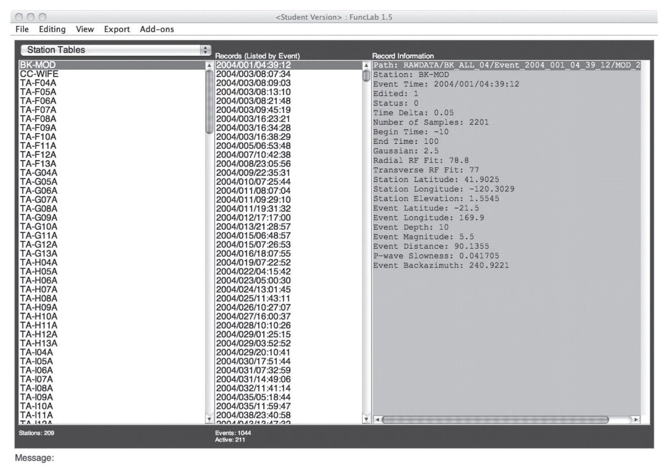
▲ Figure 2. Black and white screenshot of main FuncLab GUI. Actual FuncLab window is in color. Top-left drop-down box lists the types of tables used to organize receiver function records. Tables are listed in the left panel. Records in the selected table (highlighted in left panel) are listed in the center panel. Metadata for the selected record (highlighted in center panel) are shown in the right panel. Information about number of tables, records, and active records are listed below the left and center panels, respectively. Text displayed at the bottom is used to convey short messages to the user about ongoing or finished processes.
Trace Editor
FuncLab provides the powerful aspect of organization and efficiency through its ability to visualize many data at once. One of the main interactive visualization tools is the Trace Editor (Figure 3). The primary function of the Trace Editor is to evaluate and select waveforms efficiently for further analysis. Selecting the Manual Trace Edit GUI will read in the receiver function SAC files of the records in the selected table in the left-hand panel. Receiver functions are also normalized to the largest positive amplitude for each trace. The trace editing GUI displays the receiver functions as time series waveforms with time increasing down the y-axis and each record one unit wide across the x-axis.
Each record’s status can be changed in the GUI, allowing the user complete flexibility to specify good records that will be used in future analyses (i.e., stacking and visualization processes). Records with status “off” are not used in subsequent analyses but remain part of the dataset and are not deleted from the project. This approach has the advantage of greater freedom to perform multiple stages of trace editing or easily change the status of a record at the user’s discretion. The color of the waveform is another indicator of the record’s status. New data that have not yet been evaluated through the Trace Editor are colored red, while data previously viewed in the GUI are colored blue. All records with status “off” are shaded gray. Furthermore, right-clicking the waveform brings up a menu to start another GUI for visualizing the seismograms and radial receiver function changing the record status, and displaying event and record information useful in determining the appropriate status of the record (Figure 4).
FuncLab also allows for automated trace editing, which is currently based on two criteria, and is intended to be a first pass through a new receiver function dataset. First, a record’s status is set to “on” if the maximum amplitude after one pulse width from time zero is above a chosen threshold. The pulse width is defined as
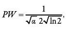
(1)
where α is the Gaussian parameter. The second criterion is a minimum fit or measure of uncertainty in the receiver function, set in the SAC header (see User Manual). All other records that do not meet these criteria are set to “off.”
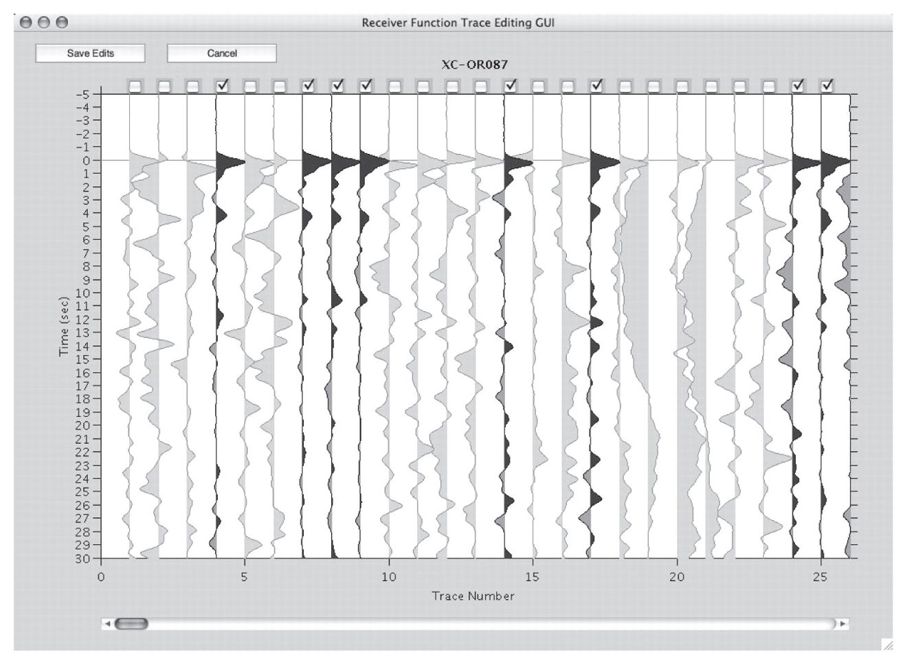
▲ Figure 3. Black and white screenshot of FuncLab Trace Editing GUI. Actual FuncLab window is in color. Waveform time series records in a selected table are displayed with colored fill denoting positive amplitudes and dark gray fill denoting negative amplitudes. Check boxes above waveforms allow the user to change the record status to "on" (selected) or "off" (unselected). Unselected records are shaded light gray. Scrollbar at the bottom allows the user to scan through all records listed in the table. The "Save Edits" button saves the record status to the project file.
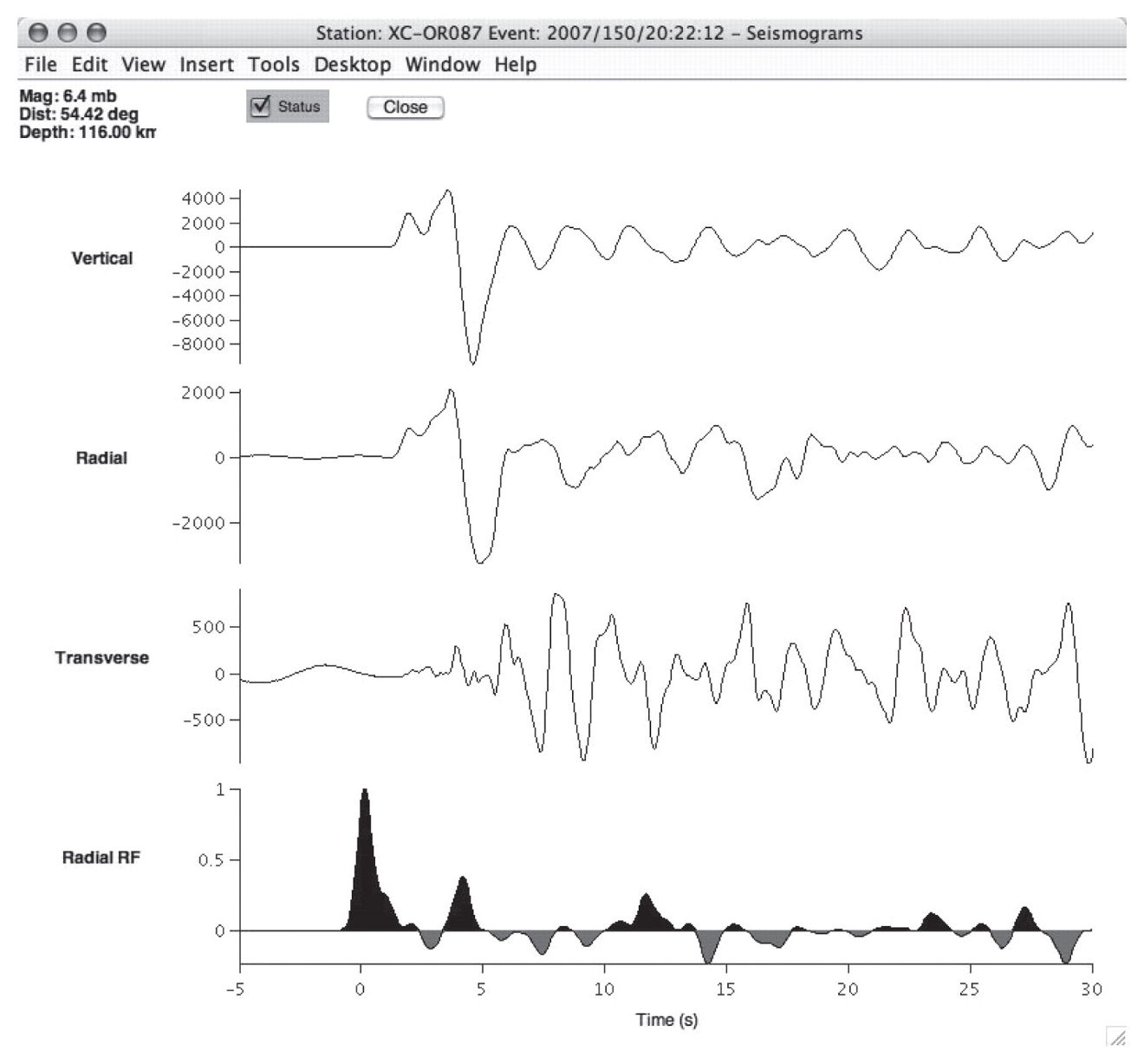
▲ Figure 4. Screenshot of trace editing system. Vertical, radial, and transverse seismograms and the associated radial receiver function are displayed. Event magnitude, distance, and depth are listed at top left. Status check box allows the user to change the record status to "on" (checked) or "off" (unchecked). This screen is accessed by right-clicking a waveform in the trace editing GUI.
Data Visualizations
A number of data plotting functions are available to help guide data analyses and are accessible from the main FuncLab GUI. Figure 5 shows three examples of the kinds of visualizations provided with this package. The Seismograms and Record Section plots (Figure 5A) display the vertical, radial, and transverse seismograms and radial and transverse receiver functions. The RF Moveout Record Section plot displays receiver function traces of active records vs. ray parameter, and the RF Moveout Image plot (Figure 5B) displays stacked records into ray parameter bins with amplitudes shown by a color scale. RF Backazimuth Record Section and RF Backazimuth Image plots (Figure 5C) are similar except that records are displayed vs. backazimuth. The Dataset Statistics visualization is not a true graph, but displays text summarizing various statistics about the dataset, such as the number of total active records. Another data coverage visualization is the Ray Parameter/Backazimuth Diagram that displays these metadata on a polar plot. Finally, two mapping options, a Station Map and a Global Event Map, are available if the MATLAB Mapping Toolbox is installed.
A log file is initiated when the project is first created within the FuncLab project and maintains information about each process performed on the dataset. The log file can be viewed from the main FuncLab GUI but is a text file that can be viewed by any text viewer. Dates and times of processes are logged, as well as the name of the process and certain preferences set to run the process. The log file should not be edited and is only intended for user guidance.
ADD-ON MODULES
FuncLab is designed to allow new analysis tools to be built around the data and metadata management environment of the main FuncLab GUI and project file. Therefore, analyses that involve stacking and other processing algorithms are included as add-on modules. The functionality of the main FuncLab GUI and trace editing GUI are not dependent upon the addons; however, each add-on must contain m-files of a certain structure, reference the metadata variables in the Project.mat file, and reference data files contained in the RAWDATA directory in order to interact with the main FuncLab GUI. In this first public release of FuncLab, we provide three built-in add-on modules of commonly employed analysis tools, including common conversion point stacking, Gaussian-weighted common conversion point stacking, and H-κ stacking. These tools can be accessed from the main FuncLab GUI and are described in more detail in this section.
Add-on modules follow a certain form and set of conventions in order to work with FuncLab. We include a set of template m-files to help users develop their own add-on FuncLab modules. Additional details regarding add-on development can be found in the User Manual.
Common Conversion Point Stacking
Common conversion point (CCP) stacking of receiver functions is a method used to image smooth regional topography on subhorizontal interfaces. It is a back-projection method in which the receiver function amplitudes are placed in the appropriate position along the raypath based on a time-to-depth conversion. These amplitudes are binned at each depth based on the position of the ray piercing point and then stacked to enhance the signal originating from that approximate position. The stacking algorithms are described in detail elsewhere (e.g., Dueker and Sheehan 1997; Eagar et al. 2010, 2011). Here, the focus is on the implementation and examples of these algorithms in FuncLab. M-files for this add-on are found in the subdirectory addons/ccp.
The CCP GUI contains editable parameters on the lefthand side and functional pushbuttons for data processing on the right-hand side. The user may set parameters for bootstrap stacking, which is a repeating process of randomly resampling the data a fixed number of times and linearly stacking receiver function amplitudes to produce a mean stack and 95% confidence interval (Efron and Tibshirani 1986, 1991). The imaging volume is defined from the latitude, longitude, and depth range input. The CCP bin spacing and width (circular radius) is also set in the parameters window. The user can specify the receiver functions to include in the stacks from ranges of both backazimuth and ray parameter. This add-on package also includes 1-D ray tracing and time-to-depth conversion that uses a chosen 1-D velocity model. Included in the package are the global 1-D models AK135 (Kennett et al. 1995), IASP91 (Kennett and Engdahl 1991), and PREM (Dziewonski and Anderson 1981). Further details on how to define other models are described within the software manual. Also included is a linear travel time correction algorithm that utilizes a seismic wavespeed tomography model to account for 3-D heterogeneities in the imaging volume. We currently provide only one regional tomography model, published in Roth et al. (2008); however, the User Manual provides details on how to define other models. Finally, a number of visualization tools, including plots of CCP bin stacks and bin histograms from bootstrapping, are accessible from the menu at the top of the CCP GUI.
The “CCP Processes” buttons are ordered to follow an established workflow for producing CCP stacked images. Subsequent processes use the matrices generated during the initial processing steps, so if the status of records changes from trace editing, the CCP Processes workflow needs to be reinitiated. The user must first perform 1-D ray tracing, which requires the maximum depth of the imaging volume, depth increment spacing, and 1-D velocity model to be set. The correction for 3-D heterogeneity is an optional step and requires the user to choose a tomography model, which can be defined or imported by the user as explained in the User Manual. The next step in CCP processing is the time-to-depth conversion of the receiver functions. This process assigns receiver function amplitudes to CCP bins at each depth increment specified by the user. The final step in the workflow is CCP stacking. The user may choose a range of backazimuths and ray parameters over which to stack, although the default is the entire dataset, from 0 to 360° and 0.04 to 0.08 sec/km, respectively. Each defined range will create a separate CCP bin stack, which allows the user to explore azimuthal and ray angle variations that may indicate complexities such as anisotropy or dipping layers. The drop-down menu in the main FuncLab GUI then allows the user to view records of CCP bins in the same manner as receiver function records.
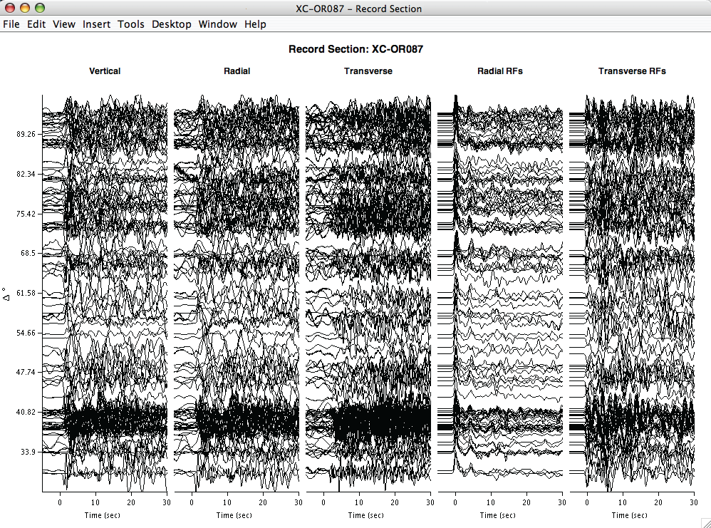
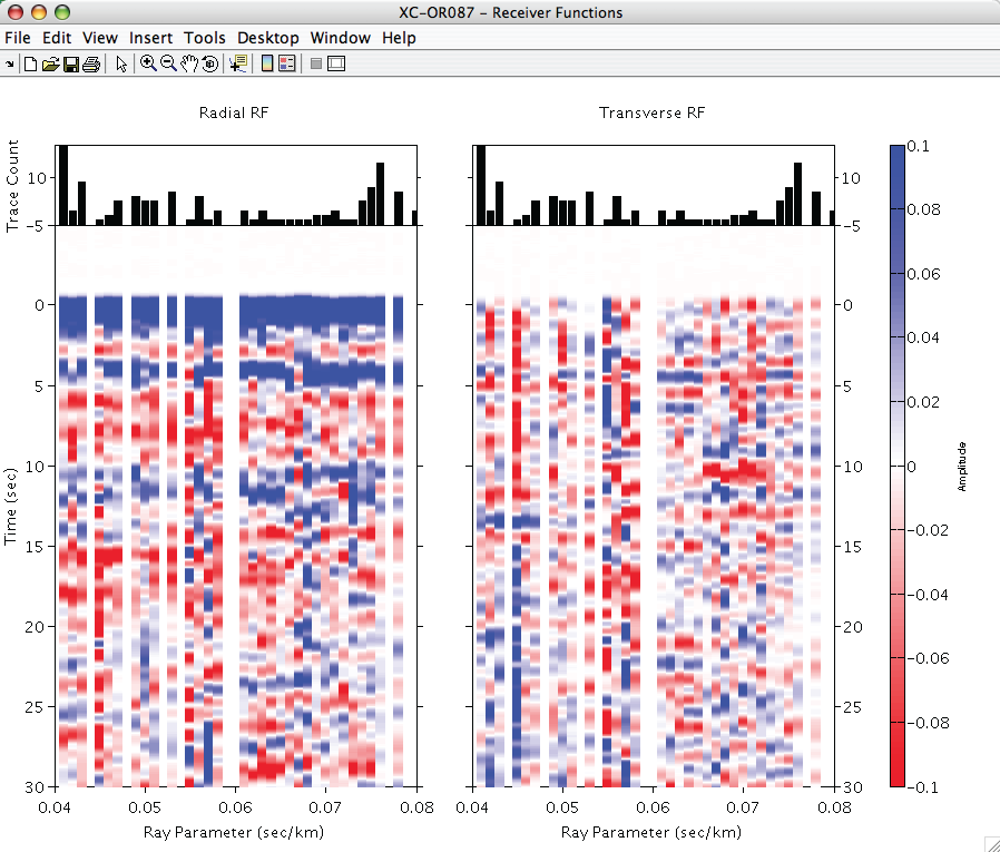
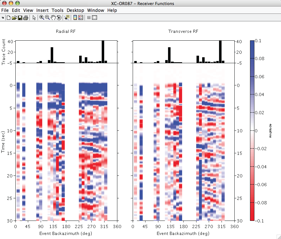
▲ Figure 5. Examples of data visualization output included in FuncLab. (A) Record section of station XC-OR087 table (data from Eagar et al. 2011), including (from left to right) the vertical, radial, and transverse time series, followed by the radial and transverse receiver functions. (B) Stacked receiver function amplitudes in ray parameter bins. Blue denotes positive amplitudes and red denotes negative amplitudes. Left panels are the radial receiver functions. Right panels are the transverse receiver functions. Top panels show histogram of receiver functions per bin. (C) Stacked receiver function amplitudes in backazimuth bins. Color and histograms are the same as in (B).
Gaussian-Weighted Common Conversion Point Stacking
Also included is an enhancement to the CCP add-on that utilizes a Gaussian weighting scheme as developed and described in Eagar et al. (2011). Gaussian-weighted common conversion point (GCCP) stacking modifies basic CCP stacking by weighting the receiver functions within the stacks by the distance of the piercing point from the image point, which is the same as the center point of the CCP bin. The weight is determined from a 2-D Gaussian function whose one standard deviation width is chosen appropriately by the array aperture and/or Fresnel zone at the imaging target. The GCCP GUI is quite similar to the CCP GUI with only a few minor differences, such as the choice of the Gaussian width and weighting function.
H-κ Stacking
H-κ stacking is a grid searching method that stacks receiver function amplitudes for a given seismic station at predicted arrival times of crustal phases based on the Moho depth (H) and Vp/Vs ratio (κ) of the crust (Zhu and Kanamori 2000). The P-to-S conversion at the Moho (Ps) and reverberations within the crust (PpPs and PpSs+PsPs) are used to reduce the inherent tradeoffs between H and κ (Zandt and Ammon 1995). Additional details of this method can be found elsewhere (e.g., Zhu and Kanamori 2000; Eagar et al. 2011).
The H-κ Stacking Analysis GUI is similar to the other add-ons described here and includes parameters that control the stacking on the left-hand side and processing functions on the right-hand side. Two options are provided for stacking and error analysis, selected from the “Error” drop-down menu. One option is a bootstrap method much like that described in the section on CCP stacking, which requires the user to set the number of times to resample and the percentage of data to resample. The other option is a linear stack, where error is determined from the contour of one standard deviation below the maximum value in the H-κ grid (Eaton et al. 2006). Several parameters that affect the resulting stack, such as the weights of the Ps, PpPs, and PpSs+PsPs phases, and the assumed Vp, can also be defined. The time, depth, and Vp/Vs parameters only affect the grid-search range and not necessarily the first-order result. As with CCP stacking, the user can specify the receiver functions included in the stack by a range of backazimuths and ray parameters. The results of these procedures are saved as separate MAT-files for each stack and store the amplitudes in the H-κ grid, the grid space axes, and the list of events that are included in the stack. Several visualizations to aid the user in the analysis are included in the package.
CONCLUSION
Receiver functions have become a commonly used imaging technique for studying sharp seismic velocity contrasts beneath seismic stations. The increase in the amount of data available to the seismological community has presented new challenges in dealing with large datasets. Here we present a new GUI-based MATLAB toolbox for organizing and analyzing receiver function data. The main FuncLab package provides a management system around which analysis tools may be written as add-on modules. We provide three add-on modules to enable common analysis techniques, including common conversion point stacking, Gaussian-weighted common conversion point stacking, and H-κ stacking. A conversion script is included to enable users to request receiver functions directly from the IRIS Data Management Center. This user-friendly environment will allow a range of researchers, from students new to seismic data analysis to seasoned scientists, to obtain useful results from receiver function analyses quickly and easily.
ACCESSING FuncLab
The FuncLab distribution is maintained at http://geophysics.asu.edu/funclab/. The MATLAB codes are packaged in a tar file for download. We also provide a User Manual for quickly getting started using the codes. Links to other supporting sources of information and data can also be found at the Web site.
ACKNOWLEDGMENTS
We thank Rick Aster and Gary Pavlis for organizing extremely helpful MATLAB tutorials on receiver functions for the 2006 IRIS/EarthScope Imaging Science Workshop at Washington University, which first inspired KCE to deal with this problem in MATLAB. We would also like to thank Mike Thorne for his original SACLAB codes (http://web.utah.edu/thorne/software.html) for importing SAC files into MATLAB, many of which were modified for use with FuncLab. Discussions with John West provided valuable insight into proper documentation and programming style. Many thanks go to Philip Crotwell (U. South Carolina), as well as Manochehr Bahavar and Chad Trabant (IRIS Data Management Center), for extensive help in providing EarthScope Automated Receiver Survey (EARS) data products that are directly compatible with FuncLab. Beta testers spent many valuable hours testing the code while in development; we would like to acknowledge those who participated, especially Eun-Sun Chong, Jonathan Delph, Chelsea Allison, Maggie Benoit, Kelsey Brunner, and Eli Raymond. This research was supported by National Science Foundation awards EAR-0548288 (MJF EarthScope CAREER grant) and EAR- 0507248 (MJF Continental Dynamics High Lava Plains grant).
REFERENCES
Andrews, J., and A. Deuss (2008). Detailed nature of the 660 km region of the mantle from global receiver function data. Journal of Geophysical Research 113; doi:10.1029/2007JB005111.
Crotwell, H. P., and T. J. Owens (2005). Automated receiver function processing. Seismological Research Letters 76, 702–708.
Dueker, K. G., and A. F. Sheehan (1997). Mantle discontinuity structure from midpoint stacks of converted P to S waves across the Yellowstone hotspot track. Journal of Geophysical Research 102, 8,313–8,327.
Dziewonski, A. M., and D. L. Anderson (1981). Preliminary reference Earth model. Physics of the Earth and Planetary Interiors 25, 297– 356.
Goldstein, P., D. Dodge, M. Firpo, and L. Minner (2003). SAC2000: Signal processing and analysis tools for seismologists and engineers. In The IASPEI International Handbook of Earthquake and Engineering Seismology, ed. W. H. K. Lee, H. Kanamori, P. C. Jennings, and C. Kisslinger, 1,613–1,614. Boston and Amsterdam: Academic Press.
Eagar, K. C., M. J. Fouch, and D. E. James (2010). Receiver function imaging of upper mantle complexity beneath the Pacific Northwest, United States. Earth and Planetary Science Letters; doi:10.1016/j.epsl.2010.06.015.
Eagar, K. C., M. J. Fouch, D. E. James, and R. W. Carlson (2011). Crustal structure beneath the High Lava Plains of eastern Oregon and surrounding regions from receiver function analysis. Journal of Geophysical Research 116; doi:10.1029/2010JB007795.
Eaton, D. W., S. Dineva, and R. Mereu (2006). Crustal thickness and Vp/ Vs variations in the Grenville orogen (Ontario, Canada) from analysis of teleseismic receiver functions. Tectonophysics 420, 223–238.
Efron, B., and R. Tibshirani (1986). Bootstrap methods for standard errors, confidence intervals, and other measures of statistical accuracy. Statistical Science 1, 54–77.
Efron, B., and R. Tibshirani (1991). Statistical data analysis in the computer age. Science 253, 390–395.
Kennett, B. L. N., and E. R. Engdahl (1991). Traveltimes for global earthquake location and phase identification. Geophysical Journal International 105, 429–465.
Kennett, B. L. N., E. R. Engdahl, and R. Buland (1995). Constraints on seismic velocities in the Earth from travel times. Geophysical Journal International 122, 108–124.
Lawrence, J. F., and P. M. Shearer (2006). A global study of transition zone thickness using receiver functions. Journal of Geophysical Research 111; doi:10.1029/2005JB003973.
Ligorria, J. P., and C. J. Ammon (1999). Iterative deconvolution and receiver-function estimation. Bulletin of the Seismological Society of America 89, 1,395–1,400.
Owens, T. J., H. P. Crotwell, C. Groves, and P. Oliver-Paul (2004). SOD: Standing Order for Data. Seismological Research Letters 75, 515–520.
Roth, J. B., M. J. Fouch, D. E. James, and R. W. Carlson (2008). Three-dimensional seismic velocity structure of the northwestern United States. Geophysical Research Letters 35; doi:10.1029/2008GL034669.
Sheehan, A. F., G. A. Abers, C. H. Jones, and A. L. Lerner-Lam (1995). Crustal thickness variations across the Colorado Rocky Mountains from teleseismic receiver functions. Journal of Geophysical Research 100, 20,391–20,404.
Suckale, J., S. Rondenay, M. Sachpazi, M. Charalampakis, A. Hosa, and L. H. Royden (2009). High-resolution seismic imaging of the western Hellenic subduction zone using teleseismic scattered waves. Geophysical Journal International 178, 775–791; doi:10.1111/j.1365-246X.2009.04170.x.
Tauzin, B., E. Debayle, and G. Wittlinger (2008). The mantle transition zone as seen by global Pds phases: No clear evidence for a thin transition zone beneath hotspots. Journal of Geophysical Research 113; doi:10.1029/2007JB005364.
Wilson, D., R. Aster, J. Ni, S. Grand, M. West, W. Gao, W. S. Baldridge, and S. Semken (2005). Imaging the seismic structure of the crust and upper mantle beneath the Great Plains, Rio Grande Rift, and Colorado Plateau using receiver functions. Journal of Geophysical Research 110; doi:10.1029/2004JB003492.
Zandt, G., and C. J. Ammon (1995). Continental crust composition constrained by measurements of crustal Poisson’s ratio. Nature 374, 152–154.
Zandt, G., S. C. Myers, and T. C. Wallace (1995). Crust and mantle structure across the Basin and Range–Colorado Plateau boundary at 37°N latitude and implications for Cenozoic extensional mechanism. Journal of Geophysical Research 100, 10,529–10,548.
Zhu, L., and H. Kanamori (2000). Moho depth variation in southern California from teleseismic receiver functions. Journal of Geophysical Research 105, 2,969–2,980.
[Back]
Posted: 03 May 2012