INTRODUCTION

The Mohorovičić discontinuity (Moho) is a globally identifiable boundary between the crust and the uppermost mantle (Dziewonski and Anderson, 1981). It is detected using seismic techniques, such as reflected energy from local earthquakes (e.g., Richards-Dinger and Shearer, 1997) or active-source experiments (e.g., Christeson et al., 2010) or from crustal reverberations of waves from distant earthquakes (e.g., Burdick and Langston, 1977; Zhu and Kanamori, 2000).

Locally, the Moho surface may exhibit complexity in terms of both the magnitude and length scale of its variations in depth; furthermore, the impedance contrast across the Moho may also vary in terms of both the magnitude and length scales (Fig. 1). Body waves and surface waves from both teleseismic and local earthquakes, as well as seismic waves from activesource experiments, may be sensitive to the variations in the Moho. These seismic waves can be used within tomographic inversions to improve the characterization of Earth’s structure in the transition from crust to upper mantle. The Moho surface constitutes an integral part of any Earth model, from regional to global scales.

The objective of this paper is to estimate a detailed Moho surface, from all available data, for onshore and offshore California; currently, no such map exists. Our motivation is to obtain a continuous, smooth surface that can be implemented within 3D structural models that are used for simulations of seismic-wave propagation (e.g., Komatitsch et al., 2004; Tape, Liu, et al., 2009), such as the California Community Velocity Model (CVM-H) of the Southern California Earthquake Center (SCEC; Süss and Shaw, 2003; Plesch et al., 2011). We first document the available datasets for estimating the Moho surface in California and its adjacent regions; we refer to this surface as the California Moho Model version 1.0 (CMM-1.0). We then describe the least-squares estimation problem of using spherical wavelets to estimate a continuous surface from the discrete data points (e.g., Tape, Musé, et al., 2009), and we also discuss the implementation of the surface within CVM-H. We also discuss relevant codes and plotting tools for utilizing the model, and the plans for future updates to the Moho surface model.

PREVIOUS STUDIES OF CRUSTAL THICKNESS IN CALIFORNIA

Mooney and Weaver (1989) created the first California-wide crustal thickness map by using data from seismic refraction/ reflection surveys, seismicity, and gravity surveys. Since 1990 the proliferation of broadband seismic stations in California has allowed for dozens of studies of crustal thickness. In this section we review local and regional studies that provide estimates of Moho depths at discrete locations.

Datasets Used in Constructing the California Moho Model

We assembled several datasets of previously published estimates of Moho depth. One important point is whether the published values refer to the crustal thickness (distance from station to Moho) or to the Moho elevation (from mean sea level to Moho). We converted all values from the published data to Moho elevation. Another issue was the choice of sign convention: we adopted a positive-downward convention, such that a “maximum Moho depth” refers to a maximal distance from the sea level to the Moho surface.

The first dataset we used was the global crustal thickness model Crust2.0 (Bassin et al., 2000), revised from Crust5.1 (Mooney et al., 1998), which provides point estimates of Moho depth on a regular grid of 2° (222 km). For our purposes, Crust2.0 is a very coarse model, but it provides at least some information in all regions, particularly in offshore regions where there are few seismic stations.

We also used the dataset of Gilbert (2012), which is a large compilation of Moho depth estimates derived using receiver functions from USArray, and also the Sierra Nevada Earth- Scope Project (Gilbert et al., 2007; Frassetto et al., 2011). The depth estimates from Gilbert (2012) are presented as a grid of bins spaced 45 km apart. We also used Moho depth estimates from the receiver function study of Yan and Clayton (2007a), which is a revised version of Zhu and Kanamori (2000). An advantage of the technique of Yan and Clayton (2007a) is that they examined receiver function stacks by azimuth, rather than stacking all receiver functions for a given station. This allowed them to detect small-scale variations in Moho topography over distances of as short as 5–10 km that exist below the stations.

▲ Figure 1. Schematic diagram illustrating five different types of variations in the Moho. The top two rows describe the topography of the surface and are the emphasis of this study. The bottom three rows describe the variations in the contrast (e.g., V_P) across the Moho; light colors represent high-wavespeed and highdensity materials, whereas dark colors represent low-wavespeed and low-density materials. In each row the other four variables are fixed; however, in reality, variations in all five could be present in a given region.

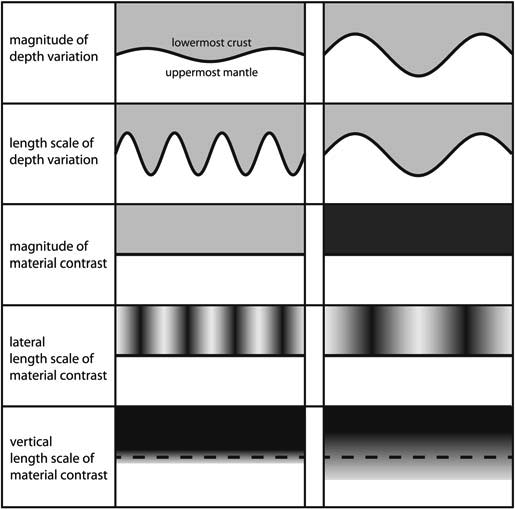
▲ Figure 1. Schematic diagram illustrating five different types of variations in the Moho. The top two rows describe the topography of the surface and are the emphasis of this study. The bottom three rows describe the variations in the contrast (e.g., V_P) across the Moho; light colors represent high-wavespeed and highdensity materials, whereas dark colors represent low-wavespeed and low-density materials. In each row the other four variables are fixed; however, in reality, variations in all five could be present in a given region.

Receiver functions are notoriously difficult to interpret in regions of large sedimentary basins, which produce reverberations that mask the desired signals from the underlying lower crust and the upper mantle. Examples of these complications have been discussed or addressed for the Denver basin (Sheehan et al., 1995), the Bohai basin in China (Chen et al., 2006), the Nenana basin in Alaska (Rossi et al., 2006), and numerous basins in California, including the Salton trough (Yan and Clayton, 2007a; Gilbert, 2012). Rather than use the highuncertainty receiver function estimates of Moho elevation near the Salton trough, the 3D model CVM-4 (Magistrale et al., 2000) adopted a uniform 22-km fixed-depth Moho surface in this region. We used this constant surface as well.

The dataset of Chulick and Mooney (2002) is, according to the U.S. Geological Survey (USGS) website (http://earthquake.usgs.gov/research/structure/crust/nam.php) where it is distributed, “a comprehensive compilation of seismic refraction and reflection data, earthquake studies, and surface wave analyses.” We supplemented this dataset with additional studies in offshore California. Legg (1991) summarized the results of seismic refraction studies in the Borderlands and the adjacent Pacific Ocean basin: “These studies showed that the Moho deepens progressively across the borderland, from about 9 to 11 at the Patton Escarpment to about 24 km at the coast and down to 32 km in the Peninsular Ranges” (p. 295). To capture the transition in crustal thickness in the offshore region, we digitized 11 published cross sections from the following papers: Keller and Prothero (1987), Miller et al. (1992), Nicholson et al. (1992), Page and Brocher (1993), Brocher et al. (1994), Lafond and Levander (1995), and Miller (2002). Additional discussion and interpretation of these active- source experiments can be found in the works of Crandall et al. (1983), Mooney and Weaver (1989), Fuis and Mooney (1990), Fuis (1998), Hole et al. (1998), Brocher et al. (1999), ten Brink et al. (2000), and Nazareth and Clayton (2003).

Additional Datasets

There were several other datasets that we considered for the estimation problem but did not use in estimating the final surface in Figure 2. Some of these datasets are redundant or inconsistent with those mentioned earlier. Others have uncertainties that we considered too large. Some of these datasets could be reconsidered in constructing future improvements to the estimated Moho surface, so we will discuss them later. The EarthScope automated receiver functions project (Crotwell and Owens, 2005) produces Moho elevation estimates for most broadband seismic stations in theUnited States. However, we instead used the published receiver function analyses of Gilbert (2012) and Yan and Clayton (2007a). Additional local receiver function studies could be considered to provide short-scale variations in Moho topography, for example, in the western Sierra Nevada (Zandt et al., 2004), San Gabriel mountains (Yan and Clayton, 2007b), eastern Mojave (Yan and Clayton, 2007a), and Piñon Flat (Baker et al., 1996). It would be useful to have a single compiled dataset containing results from such local studies.

Anomalously, deep earthquakes occur beneath the Ventura basin and the western Transverse Ranges. Bryant and Jones (1992) interpreted a maximum Moho depth of 41 km beneath theVentura basin. These depths are incompatible with receiver function estimates of Moho depth, although such estimates are notoriously difficult in the presence of major sedimentary basins (e.g., Sheehan et al., 1995).

Moho reflections from local earthquakes have been used to estimate Moho depth using the PmP (Richards-Dinger and Shearer, 1997) and SmS waveforms (Mori and Helmberger, 1996). Like receiver function studies, local body-wave studies face the challenge of a complex and unknown 3D crustal structure. In addition, the PmP and SmS arrival times depend on source parameters and lateral variations in the crustal structure, not simply the structure beneath each station, as with receiver functions.

▲ Figure 2. Estimated Moho surface for California and Nevada, including offshore regions. The circles denote data points used in the estimation problem. The solid lines are boundaries between the North America, Pacific, and Gorda plates from Bird (2003). The dashed gray line is the continental shelf, marked by the abrupt increase in bathymetric slope. The thin dashed line is the 30-km depth contour. Uncertainties associated with each data point are not plotted, although they are used in the estimation problem. The scale of wavelets used in the estimation problem ranges from q = 2 to q = 8, corresponding to length scales ranging from about 1800 to 28 km (Tape et al., 2009).

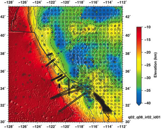
▲ Figure 2. Estimated Moho surface for California and Nevada, including offshore regions. The circles denote data points used in the estimation problem. The solid lines are boundaries between the North America, Pacific, and Gorda plates from Bird (2003). The dashed gray line is the continental shelf, marked by the abrupt increase in bathymetric slope. The thin dashed line is the 30-km depth contour. Uncertainties associated with each data point are not plotted, although they are used in the estimation problem. The scale of wavelets used in the estimation problem ranges from q = 2 to q = 8, corresponding to length scales ranging from about 1800 to 28 km (Tape et al., 2009).

Wide-angle seismic refraction surveys are capable of recording PmP waveforms. Refraction surveys, combined with reflection surveys to constrain the shallow velocity structure, can provide strong constraints on the Moho topography. We used results from refraction studies that were incorporated within the compilation of Chulick and Mooney (2002). Additional results from the Mojave region can be found in the works of Dix (1965), Gibbs and Roller (1966), Cheadle et al. (1986), and Louie and Clayton (1987). North of the Mojave, there are results from Carder (1973), Fliedner et al. (1996), Wernicke et al. (1996), Ruppert et al.. (1998), and Fliedner et al. (2000). Finally, the Los Angeles Region Seismic Experiment provided Moho estimates from the PmP and Pn arrival times (Fuis et al., 2001, 2003, 2007). Ideally, these additional results could be digitized and incorporated into a revised compilation of Chulick and Mooney (2002).

Finally, it is also possible to estimate Moho depth using gravity measurements (e.g., Romanyuk et al., 2007), seismogenic thickness (Nazareth and Hauksson, 2004), or surface wave tomography, either from earthquakes or ambient noise. Compared with seismic reflections, these observations are not as reliable as proxies for Moho topography. However, they can be used as additional constraints on estimating Moho depth in a region with seismic stations.

ESTIMATION OF A MOHO SURFACE FOR CALIFORNIA

Data and Data Uncertainties

We specified a target region bounded by latitudes 30° and 43° and longitudes −128° and −112° (Fig. 2). Assembling observations from the six datasets mentioned earlier, we obtained a set of N = 1193 observations. The N observations are represented by the data vector, d_i = h(θ_i, ϕ_i), i = 1, …, N, where θ is the colatitude, ϕ is the longitude, and h(θ,ϕ) is the elevation of the Moho surface. The minimum d_i is 6.0 km (Gorda microplate; Chulick and Mooney, 2002), and the maximum is 53.5 km (westernmost Sierra Nevada; Chulick and Mooney, 2002). This large range of values is a consequence of the transition from oceanic crust to continental crust, including former overthickened arc crust.

Data uncertainties were used within the least-squares estimation problem. In some cases the input datasets contained uncertainties; in other cases we have specified values that are proportional to the measurements. This is more sensible than assuming a constant uncertainty value for a given dataset; deeper Moho elevations are expected to have greater uncertainties, because the waves are traveling through a larger thickness of (generally unknown) crustal wavespeeds. If no uncertainties were provided, then we assigned values based on our subjective assessment; all data uncertainties can be found in the supplemental data files in the electronic supplement. The key point is that the relative differences among uncertainties have the effect of up-weighting or down-weighting the significance of each dataset in estimating the Moho surface.

Estimation of Smooth Surface Using Spherical Wavelets

▲ Figure 3. Gradient of the estimated Moho surface (Figure 2), plotted as a slope angle (equation 4). Large angles indicate sharper lateral contrasts in seismic properties (e.g., V _P, V _S, and density) across the Moho.

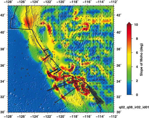
▲ Figure 3. Gradient of the estimated Moho surface (Figure 2), plotted as a slope angle (equation 4). Large angles indicate sharper lateral contrasts in seismic properties (e.g., V _P, V _S, and density) across the Moho.

We designed a multiscale estimation problem to obtain the smooth map in Figure 2. The estimation employs spherical wavelets as basis functions and was described by Tape, Musé, et al. (2009). Alternatively, one could interpolate the data using a command such as surface in Generic Mapping Tool (GMT; Wessel and Smith, 1991), which also has options to control the smoothness. The main advantage of a more general algorithm is the ability to incorporate data uncertainties (and covariances, if available) and to have better control over the regularization.

We constructed a least-squares inverse problem to minimize the sum of squared differences between observations of Moho elevation and estimates of Moho elevation. The Moho elevation was parameterized using the spherical wavelet functions whose weighting coefficients form the unknown model vector m. The model vector was given by the least-squares solution (e.g., Menke, 1989)

where G is the design matrix filled with evaluations of spherical wavelet functions at each observation point, C_D is the data covariance matrix containing data uncertainties and weighting factors, S is the regularization matrix, and λ is the regularization parameter. For details on the wavelet-based estimation problem, see Tape, Musé, et al. (2009), but note that the data in the Moho problem addressed here are 1D (elevations), whereas the data in the GPS problem addressed byTape, Musé, et al. (2009) are 3D (displacement vectors).

The solution vector m was then used to compute the Moho elevation at any input value on the sphere, a function we denote as h(θ, ϕ). Of course, uncertainties of h(θ, ϕ) will be large outside the region of input data. The surface gradient and the magnitude of the surface gradient of h(θ, ϕ) were given by

(2)

(3)

where θˆ and ϕˆ are local unit vectors pointing south and east, respectively. The magnitude of the surface gradient may be converted to a slope angle via

where R is the radius of Earth. Equation (4) is plotted in Figure 3. The slope representation of the Moho surface is helpful in predicting dynamical processes (e.g., Fay et al., 2008) because lateral gradients in material properties will be larger where the Moho slope is larger. However, caution must be taken in interpreting the slope map because it represents a derivative of the estimated surface and therefore amplifies estimated uncertainties; in other words, the slope map has greater uncertainties than that of the Moho map. Furthermore, the largest slopes will only be visible in regions with relatively dense data coverage, which allows for basis functions with shorter length scales to be considered in the estimation problem. That being said, the slope is a very intuitive quantity that helps assess the estimated surface.

In our estimation problem, regularization arises from our restriction of scales of the spherical wavelets used to estimate the continuous Moho surface. For example, wavelets with scales q = 2 and q = 8 have approximate length scales of 1,760 and 28 km, respectively (table 2 of Tape, Musé, et al., 2009). The choice of regularization leads to the estimated field having lower amplitude variations than those that are present in the observations. For example, the maximum depth of the Moho surface in Figure 2 is 39.9 km (minimum is 7.7 km below sea level), but there are input points in this focused area from Gilbert (2012) of 44 km (western Sierra Nevada) and as great as 51 km. In the extreme case, one could interpolate between all data points, which would result in a perfect fit but would produce an extremely rough—and, in many cases, unrealistic— estimated surface.

Comparison with Previous Studies

Detailed interpretations of the crustal thickness (topography elevation minus Moho elevation) variations in California can be found in the works of Yan and Clayton (2007a), Frassetto et al. (2011), Gilbert (2012), and in additional references in the References section. We have plotted our estimated surface in Figure 4 using the same color scale and region as that of Yan and Clayton (2007a) for easy visual comparison. The differences arise because (1) we use more data points and (2) we use a different estimation algorithm. Using more data points allows for coverage well outside the region of seismic stations (such as offshore California), and it allows for moderate refinements within the region of station coverage. Using a robust estimation algorithm that incorporates uncertainties, we obtained a surface that better reflects the input data. For example, the interpolated Moho map in the work of Yan and Clayton (2007a) contains some undesirable bull’s-eyes around some stations that were not present in our surface (Fig. 4); these artifacts can be eliminated with choices of regularization.

Incorporation into the California Unified Community Velocity Model

The estimated Moho surface is directly incorporated into the CVM-H 11.9 component of the Unified Community Velocity Model (UCVM) framework (Plesch et al., 2011). In the velocity model, the Moho surface separates crustal and upper mantle domains that are parameterized from distinct datasets. The crustal domain is described by a P- and S-wave travel-time tomography model after the work of Hauksson (2000), which incorporated basin velocity descriptions in the inversion. This crustal model was subsequently iterated by Tape, Liu, et al. (2009) using adjoint tomographic methods. The upper mantle domain is parameterized from a model constructed from teleseismic surface waves by T. Tanimoto (see Plesch et al., 2007). This upper mantle model is provided from 300 to 34 km below sea level, which leaves regions above the mantle model but below the new Moho surface unspecified. In CVM-H 11.9, these regions are parameterized by velocities found at the shallowest available depth in the underlying upper mantle model (34 km). Likewise, there are deep regions in the lower crust, above the updated Moho, which had not been well resolved by the crustal inversion, or had higher velocities than the underlying mantle or had been assigned to the upper mantle in previous iterations of CVM-H. These regions were identified and their velocities populated by interpolation and extrapolation from the surrounding crustal model in a manner that avoided velocity inversions at the Moho surface. Finally, all updating operations needed to be performed both on a higher resolution velocity grid, which extends down to 15-km depth, and on a lower resolution grid below 15 km, because the updated Moho surface affects both grids. During the updating procedure, attention was paid to keeping the interface between these grids consistent.

▲ Figure 4. Zoom-in of Figure 2 on southern California, plotted using the color scale of Yan and Clayton (2007a, fig. 6) to facilitate direct comparison. Active faults from Jennings (1994), plus the Kern Canyon fault (Nadin and Saleeby, 2010).

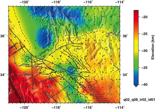
▲ Figure 4. Zoom-in of Figure 2 on southern California, plotted using the color scale of Yan and Clayton (2007a, fig. 6) to facilitate direct comparison. Active faults from Jennings (1994), plus the Kern Canyon fault (Nadin and Saleeby, 2010).

We have performed seismic wavefield simulations of 234 crustal earthquakes using CVM-H 11.9, a model that includes the estimated Moho surface shown in Figure 2 (Tape et al., 2011; Plesch et al., 2011). The 234 earthquakes were the same as those used by Tape, Liu, et al. (2009) and Tape et al. (2010) for an adjoint tomographic inversion, and the period range of interest was 2–30 s. The seismic wavefield from these crustal earthquakes is dominated by surface wave energy that is primarily sensitive to the uppermost 20 km of the crust. However, it would be possible to isolate a subset of data (i.e., waveforms) that are sensitive to changes in the Moho elevation, for example, Moho reflected waves (PmP, SmS), head waves (Pn, Sn), and Rayleigh waves with periods T > 10 s. Finally, one could compute sensitivity kernels for changes in Moho elevation; kernels for boundary topography perturbations have been discussed by Dahlen (2005) and Tromp et al. (2005) and implemented at the global scale by Liu and Tromp (2008). Future revisions to the Moho surface would benefit from an accompanying sensitivity analysis that would reveal how the changes in theMoho are expected to influence various portions of the seismic wavefield. Sensitivity analysis of waveforms generated in complex crustal models, including those sensitive to the Moho, is an area of our ongoing research.

Extracting Profiles from the Moho Surface

We provide two options for downloading the estimated Moho surface CMM-1.0. The Moho surface CMM-1.0 is integrated within the California UCVM, which is available for download from the SCEC’s website (http://scec.usc.edu/research/CVM-H). The depth to the Moho surface can also be independently queried using a code provided with the model. A triangulated mesh (T-surf ) of the Moho surface is also bundled with the model. The California UCVM provides much more information than simply theMoho surface, such as the V_P, V_S, and density values on either side of the surface.

A second option is to use a simple Matlab function, provided within the electronic supplement, to extract 2D profiles of the Moho surface. Also included is the ETOPO1 surface for topography and bathymetry (Amante and Eakins, 2009). An example output figure is shown in Figure 5.

DISCUSSION AND FUTURE IMPROVEMENTS

The fundamental assumption of this work is that there is utility in representing Moho as a smooth, continuous surface. Numerous independent datasets indicate that the Moho is a major discontinuity; indeed, the discontinuity is represented within the global Preliminary Reference Earth Model (Dziewonski and Anderson, 1981). Moho separates the continental and oceanic crust from the uppermost mantle, and therefore variations in the surface will influence short-period body waves (Pn, Sn, PmP, SmS), as well as longer-period (T > 15 s) surface waves. To accurately model seismic-wave propagation in the vicinity of the (varying) discontinuity, the Moho surface must be incorporated into finite-element meshes in such a way that element boundaries coincide with the Moho surface (Casarotti et al., 2008). Our estimated Moho for California and the adjacent regions is shown in Figure 2; this surface has been implemented within the tomographic model CVM-H 11.9 for seismic wavefield simulations (Tape et al., 2011).

▲ Figure 5. Example output from a Matlab script to generate a 2D profile of the estimated Moho surface between two input points. Also shown is the topography and bathymetry from ETOPO1 (Amante and Eakins, 2008). The variations in each surface are accentuated by allowing extreme vertical exaggeration (20:1).

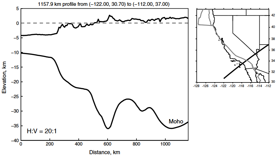
▲ Figure 5. Example output from a Matlab script to generate a 2D profile of the estimated Moho surface between two input points. Also shown is the topography and bathymetry from ETOPO1 (Amante and Eakins, 2008). The variations in each surface are accentuated by allowing extreme vertical exaggeration (20:1).

The smoothness of the resultant Moho surface (Fig. 2) may be too smooth for some purposes. There are numerous examples of relatively sharp steps in the Earth’s Moho surface, such as near the San Gabriel mountains (Yan and Clayton, 2007b) or the dramatic 22-km step in offshore southern Alaska (Christeson et al., 2010). If such blockiness of the Moho is the norm, then we would want to either allow for much shorter length scales of spherical wavelet basis functions or rather use basis functions that have sharper features (e.g., a boxcar-like Haar wavelet).

In some regions the Moho may not be seismically visible (e.g., Zandt et al., 2004; Frassetto et al., 2011). This does not diminish the utility of the geometrical representation of the surface, but it does point to the importance of defining the impedance contrast across the Moho, as well as the length scale over which the contrast occurs (Fig. 1). In the context of a 3D seismic velocity model, the Moho can effectively be eliminated by defining the same material properties above and below the Moho: The geometrical surface exists, but there is no contrast across it for seismic waves to see. An additional scenario is that there are multiple reflectors at the base of the crust (Dix, 1965). In this case, some choice must be made as to whether the estimated surface passes through either the mean of the reflectors, the uppermost reflector, or the lowermost reflector.

Future improvements to the CMM-1.0 will result from the inclusion of new or improved datasets of Moho depths. This information can readily be incorporated into the estimation problem to generate a modified Moho surface. Future efforts need to provide uncertainty estimates associated with theMoho depth estimates; these challenges partly stem from the relatively unknown uncertainties within the input data points. For now, the location of the input data points, as well as the residuals between the data and the estimated surface, provides a qualitative measure of uncertainty of the estimated surface (Fig. 2).

ACKNOWLEDGMENTS

The following datasets are available online and were used within this study: Bassin et al. (2000), Magistrale et al. (2000), Chulick and Mooney (2002), and Yan and Clayton (2007a). A text file containing all 1,193 discrete data points used in the estimation problem is provided in the electronic supplement. The figures were produced using the GMT software (Wessel and Smith, 1991). We acknowledge the helpful discussions with Egill Hauksson and Philip Crotwell. C. Tape was supported by a National Science Foundation (NSF) Postdoctoral Fellowship while at Harvard University (EAR 0848080). This research was supported by the SCEC. The SCEC is funded by NSF Cooperative Agreement EAR- 0106924 and USGS Cooperative Agreement 02HQAG0008. The SCEC Contribution Number for this paper is 1534.

REFERENCES

Amante, C., and B. W. Eakins (2009). ETOPO1 1 Arc-Minute Global Relief Model: Procedures, Data Sources and Analysis, NOAA Technical Memorandum NESDIS NGDC-24, 19 pp.

Baker, G. E., J. B. Minster, G. Zandt, and H. Gurrola (1996). Constraints on crustal structure and complex Moho topography beneath Piñon Flat, California, from teleseismic receiver functions, Bull. Seismol. Soc. Am. 86, no. 6, 1830–1844.

Bassin, C., G. Laske, and G. Masters (2000). The current limits of resolution for surface wave tomography in North America, Eos Trans. AGU 81, F897.

Bird, P. (2003). An updated digital model of plate boundaries, Geochem. Geophys. Geosyst. 4, no. 1027, doi 10.1029/2001GC000252.

Brocher, T. M., J. McCarthy, P. E. Hart, W. S. Holbrook, K. P. Furlong, T. V. McEvilly, J. A. Hole, and S. L. Klemperer (1994). Seismic evidence for a lower-crustal detachment beneath San Francisco Bay, California, Science 265, 1436–1439.

Brocher, T. M., U. S. ten Brink, and T. Abramovitz (1999). Synthesis of crustal seismic structure and implications for the concept of a slab gap beneath coastal California, Int. Geol. Rev. 41, 263–274.

Bryant, A. S., and L. M. Jones (1992). Anomalously deep crustal earthquakes in the Ventura basin, southern California, J. Geophys. Res. 97, no. B1, 437–447.

Burdick, L. J., and C. A. Langston (1977). Modeling crustal structure through the use of converted phases in teleseismic body-wave forms, Bull. Seismol. Soc. Am. 67, no. 3, 677–691.

Carder, D. S. (1973). Trans-California seismic profile, Death Valley to Monterey Bay, Bull. Seismol. Soc. Am. 63, no. 2, 571–586.

Casarotti, E., M. Stupazzini, S. J. Lee, D. Komatitsch, A. Piersanti, and J. Tromp (2008). CUBITand seismic wave propagation based upon the spectral-element method: An advanced unstructured mesher for complex 3D geological media, in Proceedings of the 16th International Meshing Roundtable, Brewer, M. L., and D. Marcum (Editors), Springer, Berlin, 579–597.

Cheadle, M. J., B. L. Czuchra, T. Byrne, C. J. Ando, J. E. Oliver, L. D. Brown, S. Kaufman, P. E. Malin, and R. A. Phinney (1986). The deep crustal structure of the Mojave Desert, California, from COCORP seismic reflection data, Tectonics 5, no. 2, 293–320.

Chen, L., T. Zheng, and W. Xu (2006). Receiver function migration image of the deep structure in the Bohai Bay basin, eastern China, Geophys. Res. Lett. 33, L20307, doi 10.1029/2006GL027593.

Christeson, G. L., S. P. S. Gulick, H. J. A. van Avendonk, L. L. Worthington, R. S. Reece, and T. L. Pavlis (2010). The Yakutat terrane: Dramatic change in crustal thickness across the Transition fault, Alaska, Geology 38, no. 10, 895–898.

Chulick, G. S., and W. D. Mooney (2002). Seismic structure of the crust and uppermost mantle of North America and adjacent oceanic basins: A synthesis, Bull. Seismol. Soc. Am. 92, no. 6, 2478–2492.

Crandall, G. J., B. P. Luyendyk,M. S. Reichle, and W. A. Prothero (1983). A marine seismic refraction study of the Santa Barbara Channel, California, Mar. Geophys. Res. 6, 15–37.

Crotwell, H. P., and T. J. Owens (2005). Automated receiver function processing, Seismol. Res. Lett. 76, no. 6, 702–709.

Dahlen, F. A. (2005). Finite-frequency sensitivity kernels for boundary topography perturbations, Geophys. J. Int. 162, 525–540.

Dix, C. H. (1965). Reflection seismic crustal studies, Geophysics 30, no. 6, 1068–1084.

Dziewonski, A., and D. Anderson (1981). Preliminary reference Earth model, Phys. Earth Planet. In. 25, 297–356.

Fay, N. P., R. A. Bennett, J. C. Spinler, and E. D. Humphreys (2008). Small-scale upper mantle convection and crustal dynamics in southern California, Geochem. Geophys. Geosyst. 9, no. 8, Q08006, doi 10.1029/2008GC001988.

Fliedner, M. M., S. L. Klemperer, and N. I. Christensen (2000). Threedimensional seismic model of the Sierra Nevada arc California and its implications for crustal and upper mantle composition, J. Geophys. Res. 105, no. B5, 10899–10921.

Fliedner, M. M., and S. RuppertSouthern Sierra Nevada Continental DynamicsWorking Group (1996). Three-dimensional crustal structure of the southern Sierra Nevada from seismic fan profiles and gravity modeling, Geology 24, no. 4, 367–370.

Frassetto, A. M., G. Zandt, H. Gilbert, T. J. Owen, and C. H. Jones (2011). Structure of the Sierra Nevada from receiver functions and implications for lithospheric foundering, Geosphere 7, no. 4, 898–921.

Fuis, G. S. (1998). West margin of North America—A synthesis of recent seismic transects, Tectonophysics 288, 265–292.

Fuis, G. S., M. D. Kohler, M. Scherwath,U. ten Brink, H. J. A. Van Avendonk, and J. M. Murphy (2007). A comparison between the transpressional plate boundaries of South Island, New Zealand, and southern California, USA: The Alpine and San Andreas fault systems, in A Continental Plate Boundary: Tectonics at South Island, New Zealand, D. Okaya,T. Stern, and F. Davey (Editors), American Geophysical Monograph 175, 307–327.

Fuis, G. S., and W. D. Mooney (1990). Lithospheric structure and tectonics from seismic-refraction and other data, in The San Andreas Fault System, R. E. Wallace (Editor), U.S. Geol. Surv. Profess. Pap. 1515, 207–236.

Fuis, G. S., T. Ryberg, N. J. Godfrey, D. A. Okaya, and J. M. Murphy (2001). Crustal structure and tectonics from the Los Angeles basin to the Mojave Desert, southern California, Geology 29, no. 1, 15–18.

Fuis, G. S., R. W. Clayton, P. M. Davis, T. Ryberg, W. J. Lutter, D. A. Okaya, E. Hauksson, C. Prodehl, J. M. Murphy, M. L. Benthien, S. A. Baher, M. D. Kohler, K. Thygesen, G. Simila, and G. R. Keller (2003). Fault systems of the 1971 San Fernando and 1994 Northridge earthquakes, southern California: Relocated aftershocks and seismic images from LARSE II, Geology 31, no. 2, 171–174.

Gibbs, J. F., and J. C. Roller (1966). Crustal structure determined by seismic-refraction measurements between the Nevada Test Site and Ludlow, California, in Geological Research 1966, U.S. Geol. Surv. Profess. Pap. 550-D, D125–D131.

Gilbert, H. (2012). Crustal structure and signatures of recent tectonism as influenced by ancient terranes in the western United States, Geosphere 8, 141–157.

Gilbert, H., C. Jones, T. J. Owens, and G. Zandt (2007). Imaging Sierra Nevada lithosphere sinking, Eos Trans. AGU 88, no. 21, 225–229.

Hauksson, E. (2000). Crustal structure and seismicity distribution adjacent to the Pacific and North America plate boundary in southern California, J. Geophys. Res. 105, no. B6, 13875–13903.

Hole, J. A., B. C. Beaudoin, and T. J. Henstock (1998). Wide-angle seismic constraints on the evolution of the deep San Andreas plate boundary by Mendocino triple junction migration, Tectonics 17, no. 5, 802–818.

Jennings, C. W. (1994). Fault activity map of California and adjacent areas, with locations and ages of recent volcanic eruptions, Calif. Div. Mines and Geology, Geologic Data Map No. 6, scale 1:750,000.

Keller, B., and W. Prothero (1987). Western Transverse Ranges crustal structure, J. Geophys. Res. 92, no. B8, 7890–7906.

Komatitsch, D., Q. Liu, J. Tromp, P. Süss, C. Stidham, and J. H. Shaw (2004). Simulations of ground motion in the Los Angeles basin based upon the spectral-element method, Bull. Seismol. Soc. Am. 94, no. 1, 187–206.

Lafond, C. F., and A. Levander (1995). Migration of wide-aperture onshore—offshore seismic data, central California: Seismic images of late stage subduction, J. Geophys. Res. 100, no. B11, 22231– 22243.

Legg, M. R. (1991). Developments in understanding the tectonic evolution of the California Continental Borderland, in From Shoreline to Abyss, R. H. Osborne (Editor), SEPM, Tulsa, Oklahoma, 291–312.

Liu, Q., and J. Tromp (2008). Finite-frequency sensitivity kernels for global seismic wave propagation based upon adjoint methods, Geophys. J. Int. 174, 265–286.

Louie, J. N., and R. W. Clayton (1987). The nature of deep crustal structures in the Mojave Desert, California, Geophys. J. Roy. Astron. Soc. 89, 125–132.

Magistrale, H., S. Day, R.W. Clayton, and R. Graves (2000). The SCEC Southern California reference three-dimensional velocity model version 2, Bull. Seismol. Soc. Am. 90, no. 6B, S65–S76.

Menke, W. (1989). Geophysical Data Analysis: Discrete Inverse Theory, Academic Press, San Diego, California.

Miller, K. C. (2002). Geophysical evidence for Miocene extension and mafic magmatic addition in the California Continental Borderland, Geol. Soc. Am. Bull. 114, no. 4, 497–512.

Miller, K. C., J. M. Howie, and S. D. Ruppert (1992). Shortening within underplated oceanic crust beneath the central California margin, J. Geophys. Res. 97, no. B13, 19961–19980.

Mooney, W. D., G. Laske, and G. Masters (1998). CRUST-5.1: A global crustal model at 5° × 5°, J. Geophys. Res. 103, 727–747.

Mooney, W. D., and C. S. Weaver (1989). Regional crustal structure and tectonics of the Pacific Coastal States; California, Oregon, and Washington, in Geophysical Framework of the Continental United States, L. C. Pakiser and W. D. Mooney (Editors), Geol. Soc. Am. Memoir, Vol. 172, 129–161.

Mori, J., and D. Helmberger (1996). Large-amplitude Moho reflections (SmS) from Landers aftershocks, southern California, Bull. Seismol. Soc. Am. 86, no. 6, 1845–1852.

Nadin, E. S., and J. B. Saleeby (2010). Quaternary reactivation of the Kern Canyon fault system, southern Sierra Nevada, California, USA, Geol. Soc. Am. Bull. 122, no. 9/10, 1671–1685.

Nazareth, J. J., and R. W. Clayton (2003). Crustal structure of the Borderland—Continent Transition Zone of southern California adjacent to Los Angeles, J. Geophys. Res. 108, no. B8, 2404, doi 10.1029/2001JB000223.

Nazareth, J. J., and E. Hauksson (2004). The seismogenic thickness of the southern California crust, Bull. Seismol. Soc. Am. 94, no. 3, 940–960.

Nicholson, C., C. C. Sorlien, and B. P. Luyendyk (1992). Deep crustal structure and tectonics in the offshore Santa Maria Basin, California, Geology 20, no. 3, 239–242.

Page, B. M., and T. M. Brocher (1993). Thrusting of the central California margin over the edge of the Pacific plate during the transform regime, Geology 21, no. 7, 635–638.

Plesch, A., P. Suess, J. Munster, J. H. Shaw, E. Hauksson, and T. Tanimotomembers of the USR Working Group (2007). A new velocity model for southern California: CVM-H 5.0, in 2007 Southern California Earthquake Center Annual Meeting, Proceedings and Abstracts, Vol. 17, 159.

Plesch, A., C. Tape, R. Graves, J. Shaw, P. Small, and G. Ely (2011). Updates for the CVM-H including new representations of the offshore Santa Maria and San Bernardino basins and a new Moho surface, in 2011 Southern California Earthquake Center Annual Meeting, Proceedings and Abstracts, Vol. 21, 214.

Richards-Dinger, K. B., and P. M. Shearer (1997). Estimating crustal thickness in southern California by stacking PmP arrivals, J. Geophys. Res. 102, no. B7, 15211–15224.

Romanyuk, T.,W. D. Mooney, and S. Detweiler (2007). Two lithospheric profiles across southern California derived from gravity and seismic data, J. Geodyn. 43, 274–307.

Rossi, G., G. A. Abers, S. Rondenay, and D. H. Christensen (2006). Unusual mantle Poisson’s ratio, subduction, and crustal structure in central Alaska, J. Geophys. Res. 111, B09311, doi 10.1029/2005JB003956.

Ruppert, S., M. M. Fliedner, and G. Zandt (1998). Thin crust and active upper mantle beneath the Southern Sierra Nevada in the western United States, Tectonophysics 286, 237–252.

Sheehan, A. F., G. A. Abers, C. H. Jones, and A. L. Lerner-Lam (1995). Crustal thickness variations across the Colorado Rocky Mountains from teleseismic receiver functions, J. Geophys. Res. 100, no. B10, 20391–20404.

Süss, M. P., and J. H. Shaw (2003). P-wave seismic velocity structure derived from sonic logs and industry reflection data in the Los Angeles basin, California, J. Geophys. Res. 108, no. B3, 2170, doi 10.1029/2001JB001628.

Tape, C., E. Casarotti, A. Plesch, and J. H. Shaw (2011). Seismogram-based assessment of the southern California seismic velocity model CVM-H 11.9 with 234 reference earthquakes, in 2011 Southern California Earthquake Center Annual Meeting, Proceedings and Abstracts, Vol. 21, 235.

Tape, C., Q. Liu, A. Maggi, and J. Tromp (2009). Adjoint tomography of the southern California crust, Science 325, 988–992.

Tape, C., Q. Liu, A. Maggi, and J. Tromp (2010). Seismic tomography of the southern California crust based on spectral-element and adjoint methods, Geophys. J. Int. 180, 433–462.

Tape, C., P. Musé, M. Simons, D. Dong, and F. Webb (2009). Multiscale estimation of GPS velocity fields, Geophys. J. Int. 179, 945–971.

ten Brink, U. S., J. Zhang, T. M. Brocher, D. A. Okaya, K. D. Klitgord, and G. S. Fuis (2000). Geophysical evidence for the evolution of the California Inter Continental Borderland as a metamorphic core complex, J. Geophys. Res. 105, no. B3, 5835–5857.

Tromp, J., C. Tape, and Q. Liu (2005). Seismic tomography, adjoint methods, time reversal, and banana-doughnut kernels, Geophys. J. Int. 160, 195–216.

Wernicke, B., R. Clayton, M. Ducea, C. H. Jones, S. Park, S. Ruppert, J. Saleeby, J. K. Snow, L. Squires, M. Fliedner, G. Jiracek, R. Keller, S. Klemperer, J. Luetgert, P.Malin, K. Miller,W. Mooney, H. Oliver, and R. Phinney (1996). Origin of high mountains in the continents: The southern Sierra Nevada, Science 271, 190–193.

Wessel, P., and W. H. F. Smith (1991). Free software helps map and display data, Eos Trans. AGU 72, no. 41, 441 ff.

Yan, Z., and R. W. Clayton (2007a). Regional mapping of the crustal structure in southern California from receiver functions, J. Geophys. Res. 112, B05311, doi 10.1029/2006JB004622.

Yan, Z., and R. W. Clayton (2007b). A notch on the Moho beneath the Eastern San Gabriel Mountains, Earth Planet. Sci. Lett. 260, 570–581.

Zandt, G., H. Gilbert, T. J. Owens, M. Ducea, J. Saleeby, and C. H. Jones (2004). Active foundering of a continental arc root beneath the southern Sierra Nevada in Californian, Nature 431, 41–46.

Zhu, L., and H. Kanamori (2000). Moho depth variation in southern California from teleseismic receiver functions, J. Geophys. Res. 105, no. B2, 2969–2980.

HOME