
Listen, Watch, Learn: SeisSound Video Products
Debi Kilb,1 Zhigang Peng,2 David Simpson,3 Andrew Michael,4 Meghan Fisher,5 and Daniel Rohrlick1
- Institute of Geophysics and Planetary Physics, University of California San Diego, La Jolla, California
- School of Earth and Atmospheric Sciences, Georgia Institute of Technology, Atlanta, Georgia
- Incorporated Research Institutions for Seismology, Washington, DC
- United States Geological Survey, Menlo Park, California
- Byrn Mawr College, Bryn Mawr, Pennsylvania
Online material: Sample SeisSound video products; MATLAB computer codes; sample data set.
INTRODUCTION TO SeisSound VIDEO PRODUCTS
The increased popularity of YouTube videos has changed the format of how information is distributed and assimilated, highlighting the importance of including auditory information in videos. Videos that include sound also permeate the research community, as evidenced by their recent increase within online supplements to journal articles. Tapping into this new approach of information exchange, we are creating videos of seismic data that augment visual imagery with auditory counterparts. We term these “SeisSound” video products (Figure 1). We find the richness and complexities of seismic data can more easily be appreciated using these SeisSound products than using just the individual visual or the auditory components independently.
Seismology includes the study of a large number of processes that affect the spectral content of a seismogram including spatial extent, duration, and directivity of a source; path effects such as attenuation, near-surface geology, and basin resonance; and the differences between abrupt tectonic earthquakes and unusual sources such as volcanic and non-volcanic tremor. With training, we can learn to discern the seismic signatures of these different processes, which can be inferred from the spectral content from time series, spectra, and spectrograms; however, subtle differences in these signals can be difficult to convey easily to a less experienced audience.
A number of our senses include the ability to act as spectral analyzers. In the audible sound range we hear pitch, in the visible light range we see color, and in the low- and sub-audible range we can feel the difference between sudden and slow motions using our senses of motion and touch. For most people, the concepts of high or low pitch (frequency) and volume (amplitude) are innate. When we listen to a symphony orchestra, we can pick out the sound of individual instruments and decipher the unique spectral content of their tones even though a hundred musicians are playing simultaneously. Similarly, we can teach people how to use these innate abilities to understand seismology by having them listen to the frequency content within a seismogram. Combining visual information with the auditory can increase the connection between the heard pitch and the visually observed frequency content within seismograms and spectrograms (see example in companion paper Peng et al. 2012, this issue, in the EduQuakes column). Introducing topics in seismology in this way can extend our ability to communicate effectively with diverse audiences who have a variety of learning styles and levels.
The audible frequency range for humans is roughly 20 Hz–20 kHz, which is about two to three orders of magnitude (or seven to ten octaves) higher than the frequency content for most recorded earthquake signals. To bring the sub-audible frequency content of earthquake seismograms into the audible range, the seismic data need to be shifted to a higher pitch. To accomplish this, the simplest and purest method is to time compress the seismogram (e.g., Hayward 1994; Dombois 2001; Dombois and Eckel 2011) by increasing the playback speed relative to the recording rate. Time compression also allows us to play back a long record in a reasonable amount of time during a lecture or demonstration.
Time compression as a method to convert seismic data to audible sound is an example of “audification,” a simple subset of the general field of “sonification,” which can involve more complex representation of data through transformations using various sound attributes (e.g., pitch, volume, and timbre). Early experiments with audification in seismology began with the advent of magnetic tape recording, which allowed playback at speeds higher than the recorded speed. One of the earliest examples of transforming seismic data into audible sounds was a recording by Benioff (1953), which includes various regional and teleseismic earthquakes recorded on an early tape system at Caltech’s Pasadena seismic station. Time compression using magnetic tape recording also was tested successfully as a method to discriminate between earthquakes and explosions (Speeth 1961; Frantti and Levereault 1965). Muirhead and Simpson (1972) used an ultra-slow speed (0.01 inch/sec) direct recording tape system to record a variety of earthquakes and explosions in Australia and incorporated time-shifted audio processing in their analysis. Some of these events were used as part of the “Murmurs of Earth” collection for the “Interstellar Record” launched on NASA’s Voyager spacecraft in 1977 (Sagan et al. 1978, 154). With the widespread use of digital recording in seismology, it is now possible to convert seismic waveforms to standard audio formats and apply simple filtering and time-compression techniques using widely available audio processing software. These types of auditory presentations of seismic data are now commonly used for educational purposes (e.g., Michael 1997; Simpson 2005; Michael 2011) and have recently regained popularity to highlight differences between typical earthquake recordings and tremor-like signals (Simpson et al. 2009; Fisher et al. 2010).
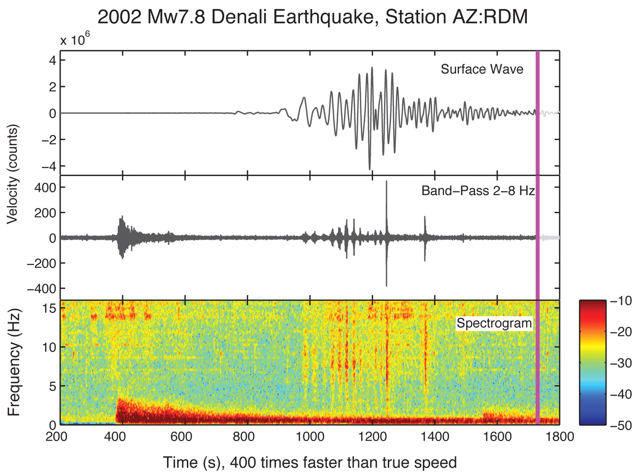
▲ Figure 1. Snapshot from a sample SeisSound video product. Shown is the transverse component of data from the 2002 magnitude 7.8 Denali earthquake in Alaska, recorded at station RDM in southern California (distance of ~4,000 km). The seismogram trace changes from light to dark as a time indicator progression line (vertical pink line) moves from left to right in the video. Original data (top). Data bandpass filtered 2–8 Hz. (middle). Spectrogram (bottom). Note the locally triggered tremors at 1,000–1,400 s that correspond to the arrival of the large amplitude surface waves (Gomberg et al. 2008; Chao et al. 2012). To remove any high-frequency artifacts introduced from using a short time window of data, we applied a 0.5 Hz high-pass filter to the data before computing the spectrogram (Peng et al. 2011).
METHOD
Overview
The SeisSound visual component includes the seismogram and corresponding spectrogram, presented in movie format indicating how the data evolve with time. An auditory sound file (WAVE format) of the data that are time compressed accompanies the visual information so the frequency content of the seismogram can be easily heard. Combining audio and visual information allows the user to both hear and see complexities in the frequency-time distribution of the seismogram that are often otherwise hidden in large-amplitude signals. These SeisSound video products provide a unique way to watch and listen to the vibration of the Earth, and help introduce more advanced topics in seismology.
Our computer codes are written with MATLAB and are freely available for use (see the electronic supplement’s MATLAB codes and data bundle). These MATLAB codes produce an audio file and a sequence of static image files. The audio track is produced using the MATLAB function wavewrite, which allows a scaling factor to be applied to speed up or slow down the playback speed. It typically takes only a few minutes for the code to process a standard seismogram. A bundled file that contains the MATLAB programs and sample data is available from our electronic supplement (MATLAB codes and data bundle). Figure 2 shows the recommended directory structure for the codes and data. A list of the MATLAB programs and a description of the parameters used to call the main program are listed in Tables 1 and 2.
For each seismogram, the MATLAB code reads seismic data in Seismic Analysis Code (SAC) format (Goldstein et al. 2003; Goldstein and Snoke 2005) and generates a sound WAVE file and the image files (~200–500) showing the evolution of the seismogram and spectrogram data with time. We use the software QuickTimePro to concatenate the images into a video and add the corresponding audio file in sync with the video to create a SeisSound video. The final SeisSound video file size (typically ~1–15 MB) is dependent on the resolution and size of the images and the total number of frames in the video. In addition to the video product, we also include a stand-alone MATLAB code sac2wav.m to directly convert seismic data in SAC format to an audio WAVE file. The Incorporated Research Institutions for Seismology (IRIS) Data Management System (DMS) also provides a Webservice for extracting waveforms from the archive and converting them to WAVE format (http://www.iris.edu/ws/timeseries/).
Steps Required to Create SeisSound Products
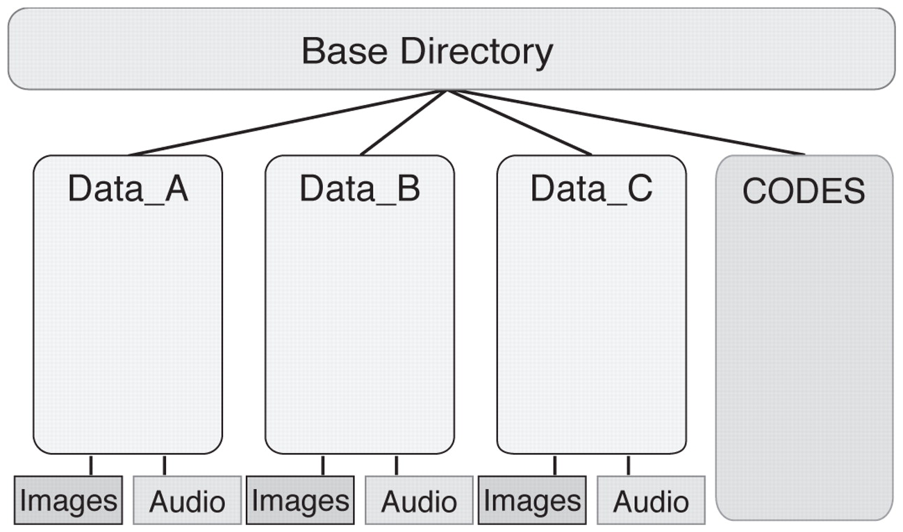
▲ Figure 2. Suggested directory structure. The “Images” and “Audio” subdirectories will be automatically added and filled by the SeisSound.m MATLAB program.
There are two main steps required to create a SeisSound video. The first step requires running the SeisSound.m MATLAB code to produce an audio WAVE file and the sequence of images. As the code runs, it will display images of the data in three panels. The top panel shows the original seismogram, the middle panel a filtered version of the data, and the bottom a spectrogram of the data (e.g., see Figure 1). If you encounter an error message indicating a missing variable or function, check that you have all of the required routines (see Table 1) and that the codes and data are stored in the proper location in the directory structure (Figure 2). If the code runs successfully, a notification of “Render Finished” will be issued at the MATLAB command window and two new subdirectories named “Audio” and “Images” will be added appropriately (e.g., see Figure 2). In the second step, the audio and image files are merged to produce a SeisSound video (Figure 3 and Table 3).
| Filename | Purpose |
|---|---|
| eqfiltfilt.m | perform a Butterworth filter |
| fget_sac.m | read sac formatted data into MATLAB |
| linex.m | draw a vertical line at a specified position |
| main_tremor.m | main program that calls SeisSound |
| sac.m | read a single SAC data file |
| sachdr.m | read the header file of SAC formatted data |
| SeisSound.m | [Main program] generated images and an audio wave file |
| sac2wav.m | create an audio wave file from SAC formatted data |
It is relatively straightforward to process seismic waveform data using SeisSound. Currently, the input data must be in SAC format and standard SAC routines or the IRIS Data Management Center (DMC) time series Webservice (http://www.iris.edu/ws/timeseries) can be used to preprocess (e.g., filter and scale) the data. Station and waveform metadata (e.g., station code, start time, sample rate, etc.) are transferred to the SeisSound program via the SAC header and additional information required to create the SeisSound products is provided via parameters in the calling function as described in Table 2.
SAMPLE SeisSound VIDEO PRODUCTS
An assortment of SeisSound examples, selected to demonstrate differences in the frequency and temporal characteristics of different seismic signals, can be found in our electronic supplement. Because of the wide dynamic range, the sound can be better appreciated on a computer with good speakers or with earbuds to hear the full effect of the lower frequencies. The amplitude of the low frequencies can sometimes be large, so it is best to keep the volume initially low to avoid damaging the speakers or, if you are using earbuds, your ears. With these SeisSound products, students can begin to decipher and understand complicated earthquake physics and earthquake triggering processes.
Notable signatures in the videos can be indicative of certain seismic processes. For example, multiple vertical streaks of red in the spectrogram, corresponding to popping sounds that begin at a fast rate and then ebb (e.g., Magnitude 8.1—Samoa Islands Region, 29 September 2009 17:48:10 UTC (station AFI); AFI_aftershock_movie60FPS.mov) are characteristic of a mainshock/aftershock sequence (e.g., Peng et al. 2006, 2007; Kilb et al. 2007). A uniform distribution of vertical streaks in the spectrogram accompanied by a repetitive pop-pop-pop tempo sound (e.g., Drumbeat earthquake swarms during the 2004 Mount St. Helens eruption; MtStHelen_Drumbeat.mov) is a characteristic of “drum beat” earthquake swarms during volcanic eruptions (Iverson et al. 2006). Another similar, yet distinctly different, signature is that of triggered deep non-volcanic tremor that typically occurs during the passage of the surface waves (e.g., Peng et al. 2008, 2009), which manifests as vertical streaks in the spectrogram during the surface wave portion of the seismic wavetrain accompanied by a relatively short-lived rat-a-tat-tat sound as from a snare drum (e.g., Triggered tremor in Parkfield, California, from the 2002 Mw 7.8 Denali, Alaska, earthquake; Denali_Triggered_Tremor.mov). The codes and example data in the electronic supplement bundled file are set up to create this example using the MATLAB script “main_tremor.m.”
| Parameter Name | Description | Default | |
|---|---|---|---|
| 1 | inputdata Data | file name | BK.PKD.HHT.SAC |
| 2 | directory | Name of the folder where the data resides and where the code generated images and audio directories will be added | Denali_2002_at_Parkfield |
| 3 | titleit | Title to be used on all generated images | Data from [name of input data file] |
| 4 | starttime | Seismogram start time in seconds, use -999 to use the start time of the data | –999 |
| 5 | endtime | Seismogram end time in seconds, use -999 to use the end time of the data | –999 |
| 6 | filt_low | Lower band limit if data filtering is requested (for low-pass only or no filter use -999) | –999 |
| 7 | filt_high | High band limit if data filtering is requested (for high-pass only or no filter use -999) | –999 |
| 8 | ff_max | Enforced maximum frequency for the spectrogram (use -999 to display all available frequencies) | –999 |
| 9 | units | Units for seismogram y-axis label (e.g., cm/s or cm/s/s). Use -999 to display no units. | –999 |
| 10 | dtype | Data type (e.g., displacement, velocity, or acceleration). Use -999 to default to data type specified in the SAC file (i.e., hdr.descrip.idep). | –999 |
| 11 | speed_factor | Audio file scale factor10012ColorBar_Upper_Limit Upper limit of the color bar of the spectrogram | 0 |
| 13 | ColorBar_Lower_Limit | Lower limit of the color bar of the spectrogram | –80 |
| 14 | FramesPerSecond | The frame per second rate you plan to use in your final SeisSound movie; this parameter will determine the number of images generated. Use -999 to let the program select the rate for you. | –999 |
AUDIENCE AND USES FOR SeisSound VIDEO PRODUCTS
We have used SeisSound video products in ~50 educational settings and public lectures ranging from teaching kindergarteners to educating more advanced audiences, including graduate students and experienced seismologists. The SeisSound images and sounds immediately captivate audiences regardless of their age and expertise, and the complexity of the message can be adjusted for each group. The innovative combination of auditory and visual information is particularly useful for introducing seismic data to beginning researchers, including upper-level undergraduate and first-year graduate students in introductory geophysics or seismology courses.
SeisSound videos can be used to highlight differences in the amplitude, frequency, and duration of P and S and surface waves and to teach how to discriminate between seismic signatures of teleseismic and local earthquakes. For the more advanced audiences, SeisSound products can be used to explore details of the spectral content in seismograms. Concepts that can be more easily discussed and investigated by incorporating sound include: categorizing seismic wave attenuation with distance from the source, discriminating between large and small earthquakes, identifying aftershock rates, and recognizing site effects including reverberation in basins (e.g., Benioff 1953; Michael 1997; Simpson et al. 2009; Fisher et al. 2010). SeisSound products can also be useful in discriminating complicated seismic signals from multiple sources, such as aftershocks within the coda of large earthquakes (e.g., Peng et al. 2006, 2007; Kilb et al. 2007), remote triggering of earthquakes (Hill et al. 1993), and tremor (e.g., Peng et al. 2008, 2009).
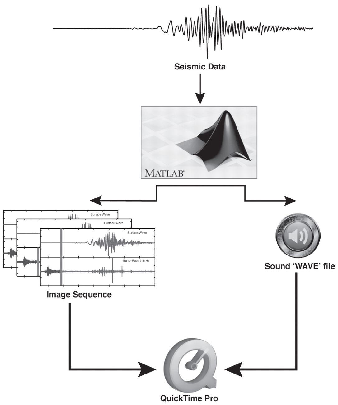
▲ Figure 3. Flow chart of the current construction of the SeisSound video products. Future plans include replacing QuickTimePro (indicated with the “Q”) with a command line freeware alternative such as ffmpeg or mencoder.
FUTURE DEVELOPMENT
We will be working with the IRIS DMC to create and distribute select SeisSound products through the IRIS product repository. To accomplish this we plan to fully automate the process of creating SeisSound video products by replacing the use of QuickTimePro with the freeware alternatives, which will allow batch mode processing. We will also design the end products to include associated metadata information such as recording station (station name and component), earthquake parameters (time, latitude, longitude, depth, magnitude), and signature of interest in the waveform (e.g., aftershocks, tremor, volcanic drumbeats).
The design of SeisSound is modular enough to easily incorporate future enhancements. These might include but are not limited to: 1) An audio-video Webservice, similar to the IRIS time series Webservice (http://www.iris.edu/ws/timeseries/), which would allow users to either specify data at the IRIS DMC that they want to process or to upload their own data; 2) A customizable display that allows the spectrograms to be displayed in log-amplitude, or shows a series of the same seismogram with different filters applied; 3) A series of different seismograms played in sequence, presented either with true relative amplitude (volume represents differences in amplitude) or normalized amplitude (each record has the same maximum level, emphasizing the diferences in pitch); 4) Aftershock/tremor location animations. Concurrent with the temporal evolution of the sound file and animated seismic data display, a map or cross-section of aftershock/tremor locations could be included where aftershocks/tremors in the current time window are marked as red or other colors, and then fade as time progresses (see example in companion paper Peng et al. 2012, this issue, in the EduQuakes column).
| StepNumber | Description |
|---|---|
| 1 | Open QuickTime Pro (http://www.apple.com/quicktime/extending/) |
| 2 | Use the top pull-down menu: File -> Open Image Sequence -> choose the first image Images/image_100.jpg, then choose 6 frames per second (or a parameter consistent with that used generating the images with SeisSound.m). An animation without sound is generated. |
| 3 | Use the top pull-down menu: File -> Open -> choose Audio/soundfile.wav. |
| 4 | Click Edit -> select all -> copy to copy the audio file into memory. |
| 5 | To add sound, first select the newly created video, and then use the pull-down menu Edit -> Add to Selection and Scale. This will add sound and scale its duration to the length of the current movie. |
| 6 | To save the final product use the pull-down menus File -> Export -> Choose “Export Movie to QuickTime Movie” and save the final movie. |
| 7 | You can preview the final SeisSound product using any viewer such as QuickTime, QuickTimePro, RealPlayer, or VLC. |
Although here we report on a relatively simple product that is primarily geared for use in educational settings, the concepts demonstrated by SeisSound can be expanded into more sophisticated research applications. A more advanced, and perhaps interactive, tool could include features such as zooming, filtering, and three-component rotation transformations. With these types of options available, the user could more efficiently search large quantities of seismic data for complicated and/or small nuances such as aftershock distribution characteristics, remotely triggered earthquakes, and tremor. We expect it will be easier to detect these key features using combined audio/visual techniques than with traditional or automated processing.
ACKNOWLEDGMENTS
We thank an anonymous reviewer and SRL Associate Editor John N. Louie for their help and guidance. Integral to the success of this project was our participation in the Southern California Earthquake Center’s Summer Undergraduate Research Experience (SCEC SURE) program, which partnered undergraduate student MF in ZP’s lab in the summer of 2010. SCEC is funded by National Science Foundation (NSF) Cooperative Agreement EAR-0106924 and U.S. Geological Survey (USGS) Cooperative Agreement 02HQAG0008. Support for this work included funding from IRIS sub-award 86-DMS funding 2011-3366 (DK) and NSF CAREER program EAR-0956051 (ZP). IRIS is funded by NSF under Cooperative Agreement EAR-0552316. The partnership with AM grew out of the online seminar series “Teaching Geophysics in the 21st Century: Visualizing Seismic Waves for Teaching and Research,” which was part of the “On the Cutting Edge—Professional Development for Geoscience Faculty” project.
REFERENCES
Benioff, H. (1953). Earthquakes around the world. On Out of This World, ed. E. Cook., side 2. Stamford, CT: Cook Laboratories, 5012 (LP record audio recording).
Chao, K., Z. Peng, A. Fabian, and L. Ojha (2012). Comparisons of triggered tremor in California. Bulletin of the Seismological Society of America 102 (2), doi: 10.1785/0120110151.
Dombois, F. (2001). Listen to seismograms: About acoustic interpretation of seismometric records. Geophysical Research Abstracts 3, 982.
Dombois, F., and G. Eckel (2011). Audification. In The Sonification Handbook, ed. T. Hermann, A. Hunt, and J. Neuhof, 301–324. Berlin: Logos Publishing House http://sonification.de/handbook/index.php/chapters/chapter12/.
Fisher, M., Z. Peng, D. W. Simpson, and D. L. Kilb (2010). Hear it, see it, explore it: Visualizations and sonifications of seismic signals. Eos, Transactions, American Geophysical Union 91, Fall Meeting Supplement, Abstract ED41C-0654.
Frantti, G. E., and L. A. Levereault (1965). Auditory discrimination of seismic signals from earthquakes and explosions. Bulletin of the Seismological Society of America 55, 1–25.
Goldstein, P., D. Dodge, M. Firpo, and L. Minner (2003). SAC2000: Signal processing and analysis tools for seismologists and engineers. IASPEI International Handbook of Earthquake and Engineering Seismology, ed. W. H. K. Lee, H. Kanamori, P. C. Jennings, and C. Kisslinger. Amsterdam & Boston: Academic Press.
Goldstein, P., and A. Snoke (2005). SAC availability for the IRIS community. Incorporated Institutions for Seismology Data Management Center, electronic newsletter https://e-reports-ext.llnl.gov/pdf/318698.pdf.
Gomberg, J., J. L. Rubinstein, Z. Peng, K. C. Creager, and J. E. Vidale (2008). Widespread triggering of non-volcanic tremor in California. Science 319, 173; doi: 10.1126/science.1149164.
Hayward, C. (1994). Listening to the Earth sing. In Auditory Display: Sonification, Audifcation, and Auditory Interfaces, ed. G. Kramer, 369–404. Reading, MA: Addison-Wesley.
Hill, D. P., P. A. Reasenberg, A. J. Michael, W. J. Arabasz, G. Beroza, D. Brumbaugh, J. N. Brune, et al. (1993). Seismicity remotely triggered by the magnitude 7.3 Landers, California, earthquake. Science 260, 1,617–1,623.
Iverson, R. M., D. Dzurisin, C. A. Gardner, T. M. Gerlach, R. G. LaHusen, M. Lisowski, J. J. Major, S. D. Malone, J. A. Messerich, S. C. Moran, J. S. Pallister, A. I. Qamar, S. P. Schilling, and J. W. Vallance (2006). Dynamics of seismogenic volcanic extrusion at Mount St. Helens in 2004–05. Nature 444, 439–443; doi:10.1038/nature05322.
Kilb, D., V. G. Martynov and F. L. Vernon (2007). Aftershock detection thresholds as a function of time: Results from the ANZA seismic network following the 31 October 2001 ML 5.1 Anza, California, earthquake. Bulletin of the Seismological Society of America 97, 780–792; doi: 10.1785/0120060116.
Michael, A. J. (1997). Listening to earthquakes. USGS; http://earthquake.usgs.gov/learn/listen/index.php.
Michael, A. J. (2011). Earthquake sounds. In Encyclopedia of Solid Earth Geophysics, 2nd ed., ed. H. K. Gupta, 188–191 New York: Springer.
Muirhead, K. J., and D.W. Simpson (1972). A three-quarter watt seismic station. Bulletin of the Seismological Society of America 62, 985–990.
Peng, Z., C. Aiken, D. Kilb, D. R. Shelly, and B. Enescu (2012). Listening to the 2011 magnitude 9.0 Tohoku-Oki, Japan, earthquake. Seismological Research Letters 83(2), 287–293.
Peng, Z., L. T. Long, and P. Zhao (2011). The relevance of high-frequency analysis artifacts to remote triggering. Seismological Research Letters 82, 856–662; doi:10.1785/gssrl.83.2.656.
Peng, Z., J. E. Vidale, K. C. Creager, J. L. Rubinstein, J. Gomberg, and P. Bodin (2008). Strong tremor near Parkfeld, CA, excited by the 2002 Denali fault earthquake. Geophysical Research Letters 35, L23305; doi:10.1029/2008GL036080.
Peng, Z., J. E. Vidale, and H. Houston (2006). Anomalous early aftershock decay rates of the 2004 M 6 Parkfield earthquake. Geophysical Research Letters 33, L17307; doi:10.1029/2006GL026744.
Peng, Z., J. E. Vidale, M. Ishii, and A. Helmstetter (2007). Seismicity rate immediately before and after main shock rupture from high-frequency waveforms in Japan. Journal of Geophysical Research 112, B03306; doi:10.1029/2006JB004386.
Peng, Z., J. E. Vidale, A. Wech, R. M. Nadeau, and K. C. Creager (2009). Remote triggering of tremor along the San Andreas fault in central California. Journal of Geophysical Research 114, B00A06; doi:10.1029/2008JB006049.
Sagan, C, F. D. Drake, A. Druyan, T. Ferris, J. Lomberg, and L. S. Sagan (1978). Murmurs of Earth: The Voyager Interstellar Record. New York: Random House, 273 pp.
Simpson, D. W. (2005). Sonification of GSN data: Audio probing of the Earth. Seismological Research Letters 76, 263 (abstract).
Simpson, D. W., Z. Peng, D. Kilb, and D. Rohrick (2009). Sonification of earthquake data: From wiggles to pops, booms and rumbles. Abstract D53E-08 presented at the 2009 Fall Meeting, American Geophysical Union, San Francisco, CA, December 14–18 (abstract).
Speeth, S. D. (1961). Seismometer sounds. Journal of the Acoustical Society of America 33, 909–916.
[Back]
Posted: 14 February 2012