|
|
Publications: SRL: EduQuakes |
EduQuakes
July/August 2009
Student Guide: Making Waves by Visualizing Fourier Transformation
Robert Smalley, Jr.
Center for Earthquake Research and Information, The University of Memphis
Online material: Additional details of the mathematics.
INTRODUCTION
Using a simple graphical presentation we can visualize the integrand of the forward and inverse Fourier transforms as a topographic surface. This presentation aids in understanding frequency domain and real-space relationships, such as the important, but often poorly understood, contribution of the frequency domain phase spectrum to the real-space shape. The Fourier transform integrand visualization method presented here can also help develop insights into complex wave behavior, such as the relationship between traveling and standing waves and the evolution of dispersing wavetrains.
BACKGROUND
Fourier analysis is often introduced with a figure showing how to approximate a function by adding together sinusoids (Figure 1(A)). I extend this presentation through the introduction of Fourier transform integrand visualization (FTIV) and use this technique to illustrate the relationship between traveling and standing waves, the Fourier shift theorem, and how the phase affects the real-space shape of a dispersing wave.
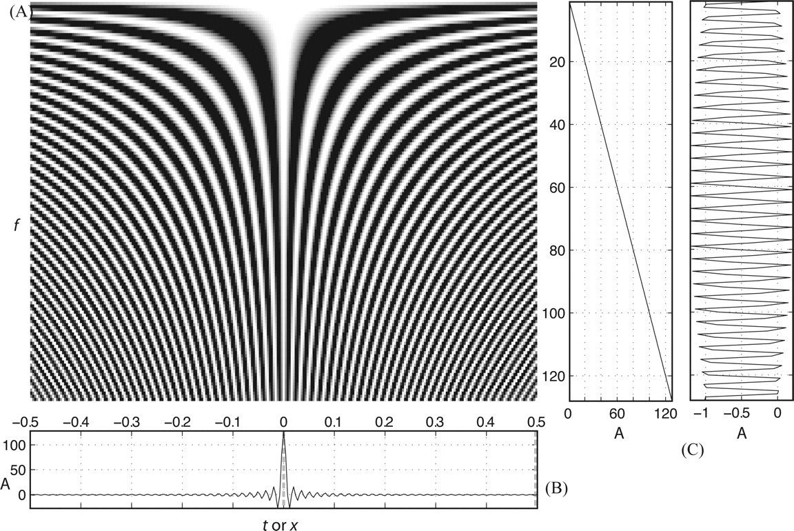
Figure 1(A) shows a real space, in this case a time-domain function, a boxcar symmetric about t = 0, and the first few terms of its Fourier series
The weights, c(ωn), and phase shifts, (φn), represent u in the frequency domain. The cos (ωnt) terms are known as basis functions and have variables from both domains, i.e., time and frequency, in their argument. The set of basis functions must meet two important conditions. First, mutual orthogonality, which means you cannot make any of them by summing the others. Second, “completeness,” which means any arbitrary function, with some conditions to ensure convergence, can be represented using only this set of functions. The Fourier series is also periodic, with period T = 2π/ω1.
The Fourier series can be generalized to the inverse Fourier transform
where the amplitude, c(ω), and phase, φ(ω), spectra come from the Fourier transform
with φ(ω) chosen to maximize |c(ω)|. (The function u(t) must be absolutely integrable and non-periodic.) The amplitude and phase spectra can be interpreted through the mathematical concept of correlation, which quantifies the similarity of functions; the Fourier transform is a correlation between the time-domain function and the time-shifted basis functions. The functions u(t) and F (ω)=[c(ω ,φ (ω))] are known as a Fourier transform pair.
VISUALIZING THE FOURIER INTEGRAND
Relating frequency-domain and time-domain behaviors, especially those related to φ(ω), is difficult with figures such as Figure 1(A), which typically use functions with φ(ω) = 0. FTIV illustrates the relationship between the Fourier transform pairs more clearly while naturally including φ(ω). Figure 2(A) (shown on the back cover) introduces the FTIV technique using the basis functions of the forward and inverse Fourier transform integrands as a topographic surface. Figure 2(B) shows the inverse Fourier transform process; following the arrows, multiply the basis functions by c(ω) to make the inverse Fourier transform integrand, then integrate to obtain the boxcar. Figure 2(C) shows the process for the Fourier transform.
The φ(ω) term in the basis function argument shifts the basis function’s position along the real-space axis (step 0, Figure 2). This is the key to FTIV that allows showing both c(ω) and φ(ω) in a clearly interpretable form. To examine the relationship between the time-domain shape and φ(ω), consider a function with Fourier transform c(ω) = 1, φ(ω)φ(ω) = 0. This makes a time-domain delta function at t = 0 (Figure 3). When c(ω) = 1, contours of the inverse Fourier transform integrand amplitude are the same as contours of constant, or stationary, argument (we will hereafter refer to the basis function argument as the “phase”), and we will equate them. This relationship makes it easier to see the phase (i.e., argument) behavior in Figures 2–5, which display the cosine of the phase and not the phase itself (a plot of the phase is not very illuminating).
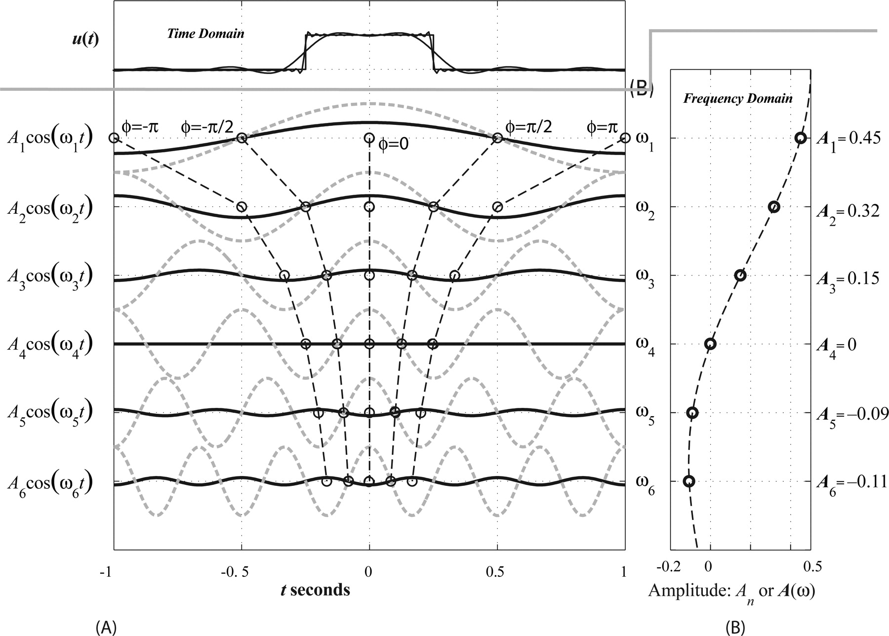
▲ Figure 1. (A) Time-domain boxcar approximations using 7 (heavy) and 100 (thin) Fourier series terms. First through sixth basis functions (gray dashed) and Fourier series terms (black). Points with stationary argument (circles) connected by vertical dashed lines between Fourier series terms become Fourier transform integrand lines of stationary phase. (B) Weights for Fourier series (circles) and Fourier transform (dashed line, scaled to match Fourier series).
The real-space function in Figure 3 is non-zero only at t = 0, where the phase is stationary. At t = 0.49, the phase varies linearly, and the integrand and running sum oscillate and remain small (zero). This observation is the basis of the principle of stationary phase: for functions that are oscillatory over most of their range, non-zero contributions to their integral come from integrand regions where the phase is stationary (e.g., Udías 1999). We will refer to the contours seen in Figure 3 as skirts. Integrating along vertical paths, constructive/destructive interference occurs where the skirts are vertical/sloping.
EXAMPLES
Traveling Waves to Standing Waves and Back
Combining two sinusoidal waves traveling in opposite directions produces a standing wave (with k as “spatial frequency”)
The right side of the equation shows a stationary wave in space, cos (kx), modulated in time by cos(ωt). Now consider two deltas propagating at ±v (Figures 4(A) and 4(B)). The inverse Fourier transform integrands of traveling sinusoidal waves and timedomain deltas move to positions x1 = ±vt1 at t1. The real-space axis is now distance (distance-domain) and the real-space plot is a snapshot of the wavefield in space. Adding the wavefields of Figures 4(A)-ii and 4(B)-ii produces the wavefield in Figure 4(C)-ii. Alternately, adding the inverse Fourier transform integrands of traveling waves in Figure 4(A)-i and 4(B)-i produces an inverse Fourier transform integrand of standing waves in Figure 4(C)-i, which integrates to the traveling deltas in Figure 4(C)-ii. How do traveling waves arise from the integration of standing waves? The right side of Figure 4(C)-i shows the inverse Fourier transform integrand decomposed into the two standing wave factors, the cos(kx) component, from x = 0 to x = 0.1 (the delta’s position), and the cos(ωt) component, from x = 0.1 to x = 0.25. At t = t1, the inverse Fourier transform is
giving the traveling deltas at x1 = ±ωt1/k = ±vt1 from the orthogonality of the cosine. The cos(ωt1) term selects positions of cos(kx), which vary with time, having the same angular frequency forming a non-oscillatory integrand ∝cos2 (kx) = cos2 (ωt1). At all other positions the integrand oscillates and integrates to zero.
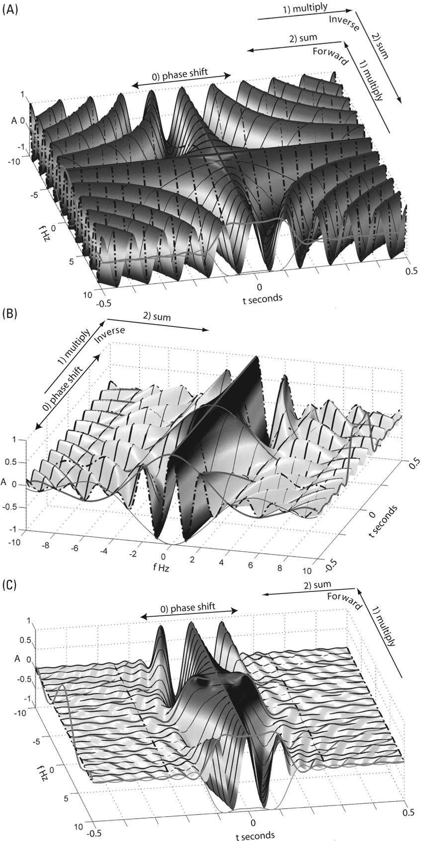
▲ Figure 2. (A) FTIV 3-D view of the common, basis function part of forward and inverse Fourier transform integrands as a surface. Frequency and time domain functions/envelopes (normalized to their maximum) shown by heavy/light plots along axes. Curves of constant amplitude and stationary phase shown on the back cover in blue. (B) Inverse Fourier transform integrand for boxcar after multiplying basis functions by c(ω). Sum parallel to f axis produces time-domain curve u(t) along t axis. (C) Forward Fourier transform integrand for a boxcar after multiplying basis functions by u(t). Sum parallel to t axis produces frequency-domain curve C(ω) along f axis.
Fourier Shift Theorem
Shifting the delta also shifts the inverse Fourier transform integrand along the real-space axis (Figures 4(A)-i and 4(B)-i), providing a graphical view of the shift theorem: a real-space shift changes φ(k) ∝ (real-space distance traveled/λ) ∝ kx , but does not change c(ω).
▲ Figure 3. FTIV gray scale topographic view of inverse Fourier transform integrand for a delta (top) with real-space function (bottom). Plots on right show running sums of the inverse Fourier transform integrand for profiles at two times or positions (gray dashed lines).
Dispersion
When velocity is a function of frequency, v(k), traveling waves change shape. Following Brune et al. (1960) and Nafe and Brune (1960), we now relate inverse Fourier transform integrand behavior to dispersion. Figure 5 (on the front cover) shows how, starting from the delta at t = 0, at t1 each inverse Fourier transform integrand component traveled x(k) = v(k)t1 to produce the inverse Fourier transform integrand (demonstrating how FTIV displays φ) and real-space wavefield shown. The vertical line of stationary phase at x = 0, t = 0 is sheared into a new shape (Figure 5(A), see cyan line on front cover) and initially sloping inverse Fourier transform integrand skirts fold and go through vertical. The wavefield also evolved into a wide, complex shape in the region v3t1 < x < v1t1, which is wider than expected from the fast and slow velocity limits, v2t1 < x < v1t1. Where does the low velocity limit, v3, come from? The answer is found by analyzing the skirt pattern.
Left of v1 and right of v3 the skirts slope, the integral is zero (Figure 5(C)-i, vi), and the real-space wave is not found. At v1, the skirt is vertical for 0 < k < α, then slopes for α < k. As regions with sloping skirts do not contribute to the integral, we can integrate over only 0 < k < α to obtain u(x, t) ∝ sinc(X) cos(k0x − ω0t), X ∝ (x − v1t)δk, (Udías 1999). This is the product of a traveling sinusoidal carrier, cos(k0x − ω0t), and a sinc modulation. The ( x − v1t ) term shifts the sinc’s location by v1t, while δk controls its width. A similar analysis can be done at v2 for δ < k. If the sinc is narrower than the sinusoids’ wavelength the result looks like a sinc pulse (x ≈ −7.5, Figure 5(B)-ii). If it is wider, the result looks like a sinusoidal wave with a sinc envelope (x ≈ 3.5, Figure 5(B)-iv). The sinc envelopes move at v1 or v2 respectively, and restrict the wavefield to finite regions containing the wave’s energy. The real-space wavefield comes from regions where the integrand’s phase is stationary (Figure 5(C)-ii and iv, gray background).
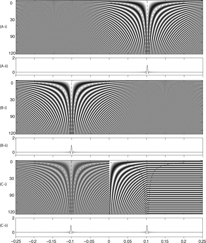
▲ Figure 4. Traveling waves in FTIV view of (A-i) and (B-i) combine into standing waves in the left side of (C-i). Solid and dashed curves in (A-i) and (B-i) show lines of stationary phase. These lines are also drawn in (C-i), where one sees a resemblance of the skirt patterns. Right side of (C-i) shows product form: a fixed spatial delta, cos(kx), modulated by cos(ωx). Real-space traveling deltas from integration if inverse Fourier transform integrands are shown in (A-ii), (B-ii) and (C-ii).
Between v1 and v2 the skirts fold. Here, waves with an observed k in the real-space wavefield, found by integrating the inverse Fourier transform integrand, do not travel at the v(k) shown by the cyan curve. They are found to travel at a velocity defined by the magenta curve (Figure 5(A)). The magenta curve connects the set of points in the inverse Fourier transform integrand having stationary phase (vertical skirts) and defines a new type of velocity, the group velocity, vg(k), at which waves (and energy, etc.) travel in the real-space. The k and v observed at position x of the real-space wave (Figure 5(B)) are the same as those associated with the point of stationary phase, (x,k) , on the magenta curve in the inverse Fourier transform integrand (Figure 5(A)). Figure 5 illustrates that phase velocity is easy to understand but hard to measure (nothing is physically traveling at the phase velocity), and that group velocity is hard to understand but easy to measure (it is the velocity of the physical wavefield we observe).
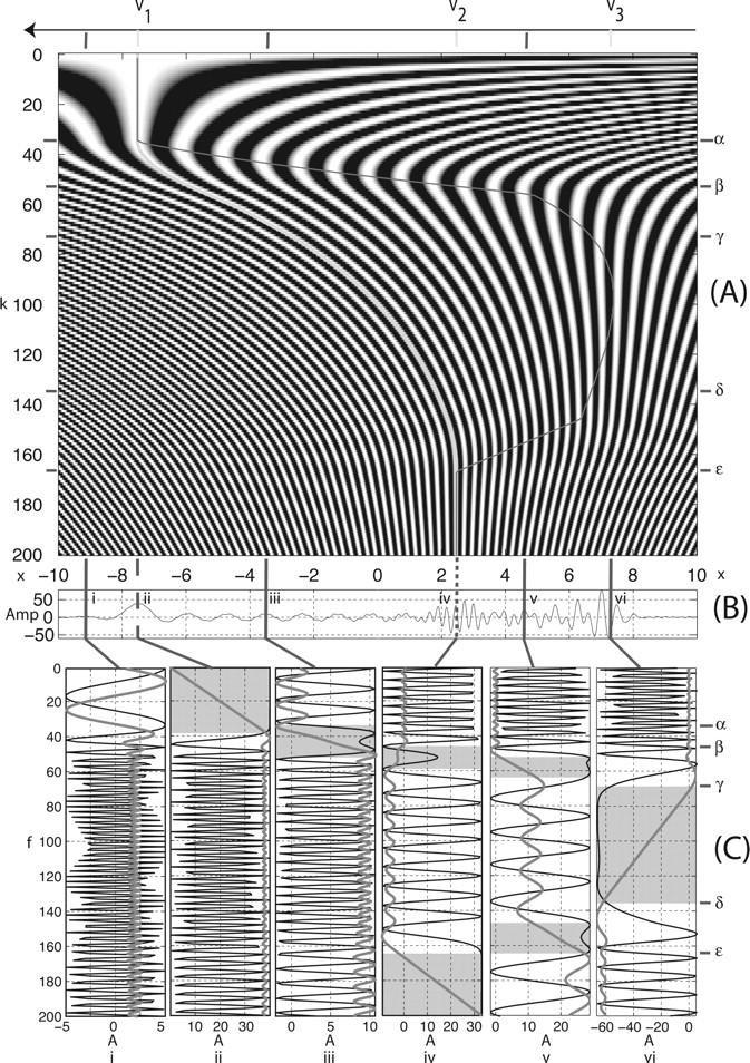
▲ Figure 5. Illustration of dispersion, phase and group velocities, and principle of stationary phase. (A) Inverse Fourier transform integrand (cos(kx − ω(k)t), v(k) = ω(k)/k) and (B) plot of dispersed wave. The distance axis, shared by inverse Fourier transform integrand and real-space plots, pans with the wave. Rescaling the x axis by 1/t1 changes it to velocity (top) with phase and group velocities shown by cyan and magenta curves on the front cover. Yellow ticks on v axis mark fast and slow limits of phase and group velocities. (C) Inverse Fourier transform integrand profiles (black, scale ±1) and running sums (red, i through vi, scale labeled). Ticks on k axis (A and C, right side) mark frequency bands for classes of real-space behavior associated with regions of stationary phase (gray background).
The inverse Fourier transform integrand skirt pattern, real-space shape, and group velocity are related by the principle of stationary phase, which applies to integrating the product of a slowly varying function and a rapidly oscillating function (see Båth 1968). In our case, the slowly varying function is c( k ) = 1 , and we only have to consider the oscillatory term, cos( kx −ω ( k )t ) , greatly simplifying the discussion without losing insight. When the phase is stationary (constant, vertical skirt),
The contribution to the wavefield from Fourier component k arrives at x at velocity vg =U( k ) . A branch of stationary phase is found between v2t1 < x < v1t1 in α < k < β, producing a sinusoidal wavefield of slowly decreasing wavelength. A running sum (Figure 5(C)-iii) shows that the largest contribution to the wavefield comes from the small region (x, k) (gray background) of the skirt pattern fold where the phase is stationary. There are two stationary phase branches in v3t1 < x < v2t1, β < k < γ and δ < k < ε, and the non-zero contributions come from the two stationary phase regions (Figure 5(C)-v). Finally, v3 is an inflection point where the second derivative of the phase is also zero, indicated by the vertical skirt in γ < k < δ that does not form a closed fold. Using an extension of the principle of stationary phase, we obtain a large amplitude pulse known as the Airy phase, associated with an extremum (minimum) of the group velocity (Figure 5(C)-vi).
DISCUSSION AND CONCLUSIONS
We have seen that φ(ω) can have significant effects on the realspace shape. How does this compare to the effects of c(ω)? The shape of the boxcar comes from c(ω). We saw that a delta with c(ω) = 1 and φ(ω) = 0 can generate a dispersed seismogram through variation of only the phase spectrum. For c(ω) = 1 and random phase, the time-domain function is white noise. The delta, white noise, and dispersed wavetrain all have c(ω) = 1, but different real-space functions determined by φ(ω), which shows that the phase spectrum carries important information and can be a major contributor to the real-space shape and its time evolution. The shape of a wave as it propagates depends on changes in both c(ω) and φ(ω). Viewing the forward and inverse Fourier transform integrands as a topographic surface provides insight into a number of real-space wavefield features such as the often underappreciated phase spectrum contribution to the real-space function, how to make traveling waves from standing waves, and the behavior of dispersing wavefields. ![]()
ACKNOWLEDGMENTS
I thank C. Langston, J. Pujol, M. Bevis, and SRL Editor L. Astiz for helpful reviews.
REFERENCES
Båth, M. (1968). Mathematical Aspects of Seismology. Developments in Solid Earth Geophysics 4. New York: Elsevier, 415 pps.
Brune, J. N., J. E. Nafe, and J. E. Oliver (1960). A simplified method for the analysis and synthesis of dispersed wave trains. Journal of Geophysical Research 65 (1), 287–304.
Nafe, J. E., and J. N. Brune (1960). Observations of phase velocity for Rayleigh waves in the period range 100 to 400 seconds. Bulletin of the Seismological Society of America 50 (3), 427–439.
Udías, A. (1999). Principles of Seismology. Cambridge: Cambridge Univ. Press, 475 pps.
Center for Earthquake Research and Information
University of Memphis
Memphis, Tennessee 38152 U.S.A.
smalley [at] ceri [dot] mempis [dot] edu
[Back]
| HOME |
Posted: 01 July 2009