
MoPaD—Moment Tensor Plotting and Decomposition: A Tool for Graphical and Numerical Analysis of Seismic Moment Tensors
Lars Krieger and Sebastian Heimann
University of Hamburg, Institute of Geophysics, Hamburg, Germany
Electronic Supplement: Software source code; examples; sample plots.
INTRODUCTION
The graphical representation of a focal mechanism as a plot of the radiation pattern on the focal sphere (sometimes referred to as “beachball diagram”) is well established. It consists of a spherical projection on a unit sphere centered at the source point of a seismic event. The sign of the P-wave radiation pattern is shown as colored areas on the sphere (as described, e.g., by Udías 1999; Stein and Wysession 2003; and Crotin 2004).
For pure shear motion on a plane, the focal sphere may be fully described by the angles of strike, dip, and slip-rake of this fault plane (cf., Shearer 1999; Aki and Richards 2002). In this case the construction of the spherical projection into the ![]() is straightforward (e.g., Stein and Wysession 2003, chapter 5).
is straightforward (e.g., Stein and Wysession 2003, chapter 5).
Several tools are available to do this work. They exist either as a more or less configurable, independent software package (Snoke 2003; Srivastava et al. 2006; Luis 2007; Haeussler and Labay 2007), as supplements for GMT, MATLAB (Creager 1997; Center for Earthquake Research and Information 2008) or Mathematica (Scherbaum et al. 2010), or as an online applet (Helffrich 2007). Almost all of the existing software consider only these pure shear cracks. The visualisation of a more complex source mechanism, e.g., an arbitrary seismic moment tensor with six independent entries, is often not possible.
Only a few tools exist at all that can handle this general case. The most commonly used one is the psmeca-tool in GMT (Wessel and Smith 1999). However, projections for arbitrary viewpoints are not possible with psmeca.
We present the free platform-independent command line tool MoPaD, written in the Python programming language that allows one to generate, plot, and save scale- and case-independent focal spheres in a variety of standard graphic formats. The tool allows the use of GMT for plotting focal mechanisms even in the above mentioned cases by using the GMT program psxy.
As an additional feature, the moment tensor can be decomposed and transformed into different representations. Alternatively, the core functionality of MoPaD is provided as a Python library.
After providing the theoretical basis in the next section of this paper, we will turn to the technical aspects of implementation. We give a short introduction into the handling of MoPaD and its methods by examples in the last section.
THEORY
Many publications describe in detail the theory of source mechanisms (Udías 1999) but do not fully cover their visualisation. The idea of constructing focal spheres is mainly sketched from a geometrical point of view in the case of double-couple sources (cf., Stein and Wysession 2003) or handled as a contour plot of first arrival polarizations (e.g., Riedesel and Jordan 1989).
We start with the description of the stable construction of a general focal sphere diagram (FSD) on the basis of an analytical approach. This is based on the calculation of nodal lines on the focal sphere.
Definitions and Terminology
The seismic moment tensor M is defined in the form of a realvalued symmetric 3×3 matrix. It is fully diagonalizable, so its characteristics are completely determined by its eigensystem with the eigenvalues {σP ≤ σN ≤ σT}. The corresponding eigenvectors are the pressure-, null-, and tension-axis. This orthogonal principal axis system is used to derive an exact description of the FSD.
With M := (M11, M22, M33, M12, M13, M23) there is a bijection ![]() . According to this mapping, M is identified with M for the remainder of this publication.
. According to this mapping, M is identified with M for the remainder of this publication.
Within the following steps, we take advantage of a planar reflective symmetry. The eigenvector that corresponds to the largest absolute eigenvalue is the symmetry plane’s normal vector for all cases except two in which the source has a significant volumetric component. To handle these exceptions, we introduce the exception-value χ, using the reduced eigenvalues of M ![]() :
:
Accommodating the mentioned symmetry, we introduce the nomenclature
where the π denotes the pairwise permutation function π : (a,b)![]() (b,a), which is applied if the exception-value is nonzero. The eigenvalue σΣ defines the symmetry, where Σ is its respective eigenvector. The second eigenvector N remains unchanged and the third is denoted by H (cf. Figure 1).
(b,a), which is applied if the exception-value is nonzero. The eigenvalue σΣ defines the symmetry, where Σ is its respective eigenvector. The second eigenvector N remains unchanged and the third is denoted by H (cf. Figure 1).
Nodal Lines
The P-wave radiation pattern is characterized by nodal lines of the polarity of the first arrivals on a unit sphere around the origin on the focal sphere, and we are interested in a closed formula describing these lines.
In the basis system HNΣ, the focal sphere is planar symmetric with respect to the HN-plane, so the lines are given by a closed curve around the positive Σ-axis (shown in Figure 1) and its reflection on the symmetry-plane.
As a start we calculate the net particle displacement u(P) for every point P := (x, y, z) on the focal sphere. For a general solution, the coordinates are expressed in terms of the eigenvector basis HNΣ. Due to the symmetry, only points in the upper hemisphere are considered; so P = (xH, yN, zΣ) with zΣ ≥ 0. Following this notation, one obtains for the oriented particle displacement u* at P

The effective net particle displacement, pointing radially outward, is obtained by projecting the displacement vector u* onto the position vector, expressed via the scalar product
which can be read as

The nodal lines are defined by u(P) = 0. In spherical coordinates, with φ ∈ [0, 360°[ being the azimuthal angle between N and the horizontal projection of P to the HN-plane, one obtains an explicit function for the polar opening angle α between Σ and P. This yields the desired description of the two lines around the positive (α+) and negative (α−) part of the Σ-axis in a closed, yet parametrized form:
The most frequently occurring types pure double couple (σΣ = −σH, σN = 0) and pure compensated linear vector dipole (CLVD) (σH = σN = −1/2σΣ) are special cases of this general solution. If the isotropic part of the moment tensor outweighs the deviatoric content, the discriminant in the right hand side of Equation 6 becomes negative, so that no nodal lines can be defined. This leads to a uniformly colored focal sphere, consistently reflecting the constant sign of the radial particle displacement.
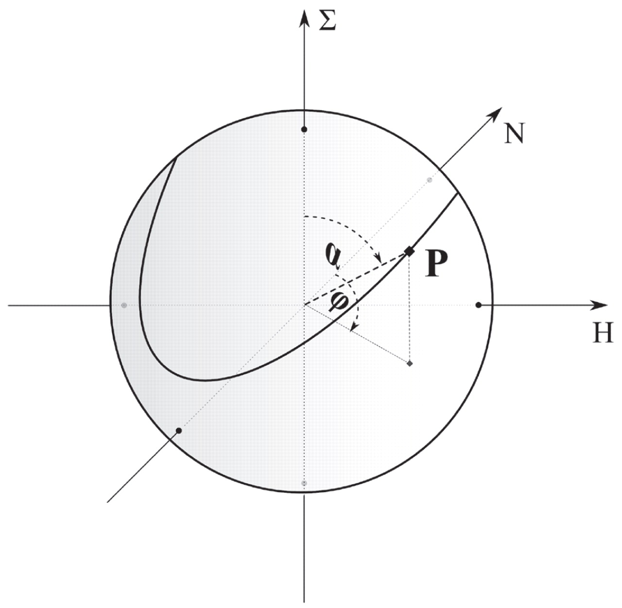
▲ Figure 1. Point P(α, φ) on the “positive” nodal line in the HNΣ-system.
Transformation
A solution in an abstract eigenvector system and its uniqueness is quite satisfactory from a theoretical point of view. For plotting, an arbitrary basis system of the ![]() and a suited projection onto an
and a suited projection onto an ![]() -plane are required.
-plane are required.
Having a basis-independent solution for the curve, we append a transformation into the desired basis system to plot the projection of the sphere and all nodal lines. The output can be given in all implemented basis systems (see Table 1). In the following, M is given in north, east, down (NED), unless otherwise noted.
Projections 
Three projection algorithms are implemented; the tangential stereographic projection is set as default. Other possibilities are lambert azimuthal equal-area and orthographic projection (cf. Bronstein and Semendjajew 1987). Figure 2 illustrates the differences between the projections.
In MoPaD it is possible to define which hemisphere shall be projected. The standard back-hemisphere projection can be changed into a front-hemisphere projection; thereby the roles of upper and lower hemisphere (as well as the respective projection poles) are interchanged.
| TABLE 1 Basis Systems Supported by MoPaD |
|||
|---|---|---|---|
| Short | Basis vectors | Usage | |
| NED | North, East, Down | Jost and Herrmann | Jost and Herrmann 1989 |
| USE | Up, South, East | Global CMT Catalog | Larson et al. 2010 |
| XYZ | East, North, Up | general formulation | Jost and Herrmann 1989 |
| RT | Radial, Transverse, Tangential | psmeca (GMT) | Wessel and Smith 1999 |
| NWU | North, West, Up | Stein and Wysession | Stein and Wysession 2003 |
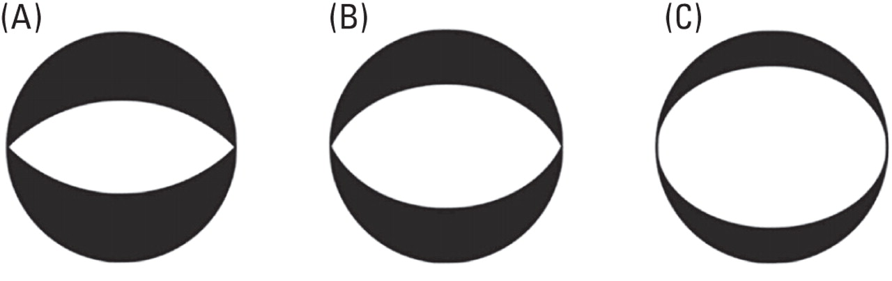
▲ Figure 2. The FSD for M = (1, 0, -1, 0, 0, 0) in A) stereographic, B) Lambert, C) orthographic projection.
Viewpoint
Figure 3 illustrates the option to transform the viewpoint. The view on the focal sphere solution is defined by three angles. The two angles θ and φ define the observer’s position in relation to the sphere, and Ω sets the viewing angle (azimuth) with respect to a local North N’. A common FSD is set up so that one looks from above the center (θ = 0, φ = 0), while local North is on the upper edge of the plot (Ω = 0).
For changing the viewpoint to V’, a local coordinate system is set up at this new position. The negative position vector defines the local Down = D’, while local North = N’ is obtained by an orthonormalization of D’ and N (Gram-Schmidt method). Finally, an outer product of the first basis elements yields E’. The set N’E’D’ provides a right-handed local basis of the ![]() . Within this local system, the rotation according to the provided azimuthal angle is carried out. The projection and plotting is referenced to this new system.
. Within this local system, the rotation according to the provided azimuthal angle is carried out. The projection and plotting is referenced to this new system.
Example
We take a closer look at an arbitrarily chosen source mechanism, defined by M = (1, 2, 3, –4, –5, –10).
In Figure 4A, the upper hemisphere of the FSD is shown as seen from above (viewpoint (0,0,0)); four additional viewing positions (a–d) for vertical sections are indicated. The center plot of Figure 4B illustrates the standard vertical view on the lower (back) hemisphere from above the source in stereographic projection. It was generated with the MoPaD command
mopad plot 1,2,3,-4,-5,-10 .
Apart from that, the FSDs a–d visualize the respective vertical back hemispheres that have been generated with the viewpointoption arguments (a:{90,0,180}, b:{0,–90,–90}, c:{–90,0,0}, d:{0,90,90}).

▲ Figure 3. Changing the viewpoint from V to V’ (θ, ϕ, Ω) with its new local basis N’E’D’.
Decompositions
Within MoPaD, four possibilities to decompose a moment tensor into different components are available:
- Isotropic + double couple + CLVD,
- Isotropic + major double couple + minor double couple,
- Isotropic + three double couples, and
- Isotropic + CLVD + strike-slip movement + dip-slip movement.
The definition and nomenclature of the first three decompositions follow directly (Jost and Herrmann 1989). The fourth alternative is described in Dahm (1993). The definition of the scalar seismic moments is given in Bowers and Hudson (1999).
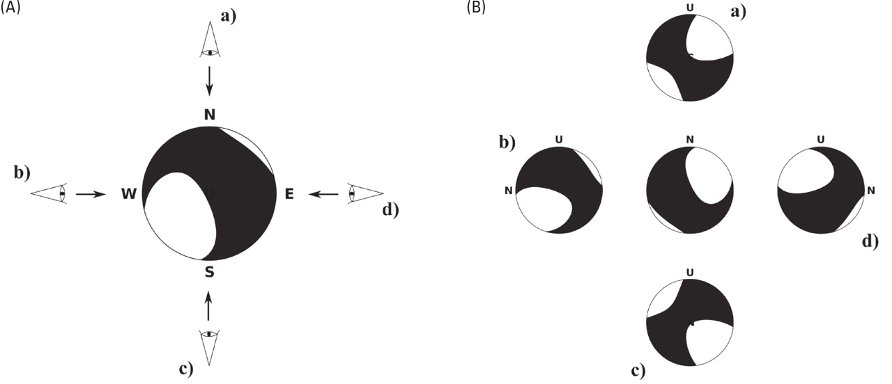
▲ Figure 4. (A) The nonstandard view on a focal sphere’s upper hemisphere (M = (1, 2, 3, -4, -5, -10)). Five additional important viewing positions (North, West, South, East and Up) are indicated. (B) The FSDs of the respective back hemispheres are shown for the five positions stated in A.
IMPLEMENTATION
MoPaD is written in Python and can be used as a Python module or from the command line. In addition to the Python standard installation, the modules numpy (Oliphant 2006) and matplotlib (Hunter 2007) are required.
Developed under the GNU Lesser General Public License (LGPL), MoPaD is designed as an open-source tool.
For use as a command line tool, MoPaD is subdivided into four methods:
- plot
- This method is the main feature of MoPaD; it returns a plot of an FSD in several graphic formats. The theoretical shape of the diagram, obtained as described above, is transformed according to given options. After the consecutive projection, a visualisation is provided using the module matplotlib (Hunter 2007).
- describe
- A brief overview of the provided source mechanism can be obtained using this method. Both the moment tensor representation as well as the orientation of the main shear component are shown.
- decompose
- Returns strings containing information about the components of the original source mechanism. Either a full or a partial decomposition of the internally calculated seismic moment tensor can be returned in different basis systems.
- gmt
- A string is returned containing
 -coordinates in (x, y)-form, which can be fed into the psxy function of GMT.
A combination of methods decompose and plot allows, for instance, for the graphical decomposition of a moment tensor, as shown in Figure 5.

▲ Figure 5. Graphical decomposition of M := (1, 2, 3, -4, -5, -10) into its isotropic and deviatoric components: the latter is further decomposed into double couple and CLVD. Percentages of the parts are shown. The graphical scaling is linear in area.
EXAMPLES
In order to demonstrate the main features of the methods of MoPaD, we present here some small example applications. (All input has to be provided as one line, all linebreaks in the following examples are due to the proper typesetting of this article.)
- plot
- In addition to the case presented previously for a varying viewpoint, where we got a very simple plot, we give here an input line for calling MoPaD that contains a combination of options. In contrast to the aforementioned case, this plot is not shown but stored directly into a file:
mopad plot 1,2,3,-4,-5,-10 -s 10 -v -50,30,-0 -U -p o -f FSD_complex.svg
-r 252,233,79 -w 117,80,123 -d 1 3 red 0.5 -e 15 4 1 -b
With this input, we have chosen to plot the deviatoric part of the moment tensor with an output size (-s) of 10 cm, a view (-v) from south-east showing the front hemisphere (-U), the orthographic projection (-p), an .svg formatted output file (-f), the tensional area in yellow (-r), and the pressure domain in purple (-w). Additionally, one fault plane of the governing double-couple part is superimposed (-d), and the positions of eigenvectors (-e), as well as the axes of the basis system (-b), are indicated. (The generated file is provided in the electronic supplement of this publication.)
This setup is a highly unusual combination for an everyday focal sphere visualisation, but it serves the purpose to show the action of an arbitrary set of options.
- describe
- The method describe provides a fast and simple way to obtain an overview of all parameters of M. In addition, it enables an easy conversion between basis systems (options -i and -o define input and output basis):
mopad describe 1,2,3,-4,-5,-10,7.2e15 -o USE
Scalar Moment: M0 = 1.07302e+17 Nm (Mw = 5.3)
Moment Tensor: Muu = 0.216, Mss = 0.072, Mee = 0.144, Mus = -0.360, Mue = 0.720, Mse = 0.288 [ x 1e+17 ]
Fault plane 1: strike = 337°, dip = 85°, slip-rake = 105°
Fault plane 2: strike = 84°, dip = 16°, slip-rake = 18°
- decompose
- The moment tensor can be decomposed into different parts. Here we use a partial (-p) decomposition of M = (1, 2, 3, –4, –5, –10) in order to determine the double-couple part and isotropic component, including the respective percentages:
mopad decompose 1,2,3,-4,-5,-10 -p dc,dc_perc,iso,iso_perc

Double-Couple part in NED-coordinates:
/ -1.77 -1.95 -2.97 \
| -1.95 0.41 -7.30 |
\ -2.97 -7.30 1.36 /

Double-Couple percentage:
55

Isotropic part in NED-coordinates:
/ 2.00 0.00 0.00 \
| 0.00 2.00 0.00 |
\ 0.00 0.00 2.00 /

Isotropic percentage:
13
- gmt
- MoPaD’s gmt-method provides the coordinates of the nodal lines of the FSD, as well as the eigenvectors. These are to be piped into the psxy-tool of GMT. The tension-areas of the FSD hold the color-key “1” for the psxy-Z-option; the pressure areas the key “0.” If requesting only the border lines, the key is also set to “1.”
The complete command for generating the FSD in Figure 4B (center) by using a combination of MoPaD and GMT is:
mopad gmt 1,2,3,-4,-5,-10 -t fill -p s | psxy -Jx4/4 -R-2/2/- 2/2 -P
-Cpsxy_fill.cpt -M -K -L >BB1.ps && mopad gmt 1,2,3,-4,- 5,-10 -t lines
-p s | psxy -Jx4/4 -R-2/2/-2/2 -W5 -P -Cpsxy_lines.cpt -M -O >> BB1.ps
(The GMT color tables psxy_lines.cpt and psxy_fill.cpt must be generated externally.) That seems to be rather complicated, but the high flexibility of MoPaD proves beneficial in the case of handling focal mechanisms, which are not limited to the standard view and projection. There the commands are not more complex than in the standard case:
mopad gmt 1,2,3,-4,-5,-10 -t fill -p o -v 45,45,45 | psxy -Jx4/4
-R-2/2/-2/2 -P -Cpsxy_fill.cpt -M -K -L > BB2.ps && mopad gmt
1,2,3,-4,-5,-10 -t lines -p o -v 45,45,45 | psxy -Jx4/4 -R-2/2/-2/2 -W5 -P
-Cpsxy_lines.cpt -M -O >> BB2.ps
This yields a rotated FSD (viewpoint 45°, 45°, 45°) in the orthographic projection. (The files BB1.ps and BB2.ps, as well as the color table files, can be found in the electronic supplement.)
CONCLUSIONS
The tool MoPaD provides a variety of plotting options for the widespread focal mechanism’s graphical representation, visualizing seismic source mechanisms.
The concept given in the Theory section allows for a fast and easy plotting of the FSDs, independent of the source type, orientation, and viewpoint of the observer. In this way, the tool represents a significant improvement for everyday work in seismology. Yielding a simplification for creating arbitrary FSDs in combination with GMT’s psxy, MoPaD can be a useful supplement.
The software is open source, and a first alpha version is freely available from the electronic supplement for this publication. More recent versions will be available on the homepage of MoPaD: http://www.mopad.org. An instruction manual with descriptive examples is provided there together with the source code. MoPaD is additionally integrated into ObsPy, a Python toolbox for seismology (Beyreuther et al. 2010).
ACKNOWLEDGMENTS
The development of this new tool was initiated by the lack of easy to use stand-alone tools for plotting general focal mechanisms, not restricted to pure double couples. More intuitive manuals within the seismological community are highly desirable. Moreover, the need for an appropriate Python-module for this purpose was a further motivation. The authors thank their supervisor, Professor Dahm at the Institute of Geophysics at the University of Hamburg, for his idea to implement MoPaD’s gmt-method, providing the connection to psxy, as well as the fourth non-standard decomposition of the moment tensor. Thanks go also to Stefan Trabs for testing the software.
REFERENCES
Aki, K., and P. G. Richards (2002). Quantitative Seismology, 2nd ed. Sausalito, CA: University Science Books.
Beyreuther, M., R. Barsch, L. Krischer, T. Megies, Y. Behr, and J. Wassermann (2010). ObsPy: A Python toolbox for seismology. Seismological Research Letters 81 (3): 530.
Bowers, D., and J. A. Hudson (1999). Defining the scalar moment of a seismic source with a general moment tensor. Bulletin of the Seismological Society of America 89 (5): 1390.
Bronstein, I. N., and K. A. Semendjajew (1987). Taschenbuch der Mathematik. Thun und Frankfurt am Main: Verlag Harri Deutsch.
Center for Earthquake Research and Information (CERI) (2008). A MATLAB routine for handling beachballs. http://www.ceri.memphis.edu/people/olboyd/Software/bb.m. Date retrieved: 24 July 2010. Date last modified: 28 March 2008.
Creager, K. (1997). Coral. Seismological Research Letters 68 (2): 269–271. http://earthweb.ess.washington.edu/creager/coral_tools.html.
Cronin, V. (2004). A Primer on Focal Mechanism Solutions for Geologists. http://serc.carleton.edu/files/NAGTWorkshops/structure04/Focal_mechanism_primer.pdf. Date retrieved: 24 July 2010.
Dahm, T. (1993). Relative moment tensor inversion to determine the radiation pattern of seismic sources (in German). PhD thesis, Geophysikalisches Institut, Universität Karlsruhe.
Haeussler , P. J., and K. A. Labay (2007). 3D Visualization of Earthquake Focal Mechanisms Using ArcScene®. http://pubs.usgs.gov/ ds/2007/241/. Date retrieved: 26 July 2010. Date last modified: 17 December 2007.
Helffrich, G. (2007). Focal mechanisms. http://www1.gly.bris.ac.uk/~george/focmec.html. Date retrieved: 24 July 2010. Date last modified: 9 June 2007.
Hunter, J. (2007). Matplotlib: A 2D graphics environment. In Computing in Science & Engineering, 90–95.
Jost, M. L., and R. B. Herrmann (1989). A student’s guide to and review of moment tensors. Seismological Research Letters 60 (2), 37–57.
Larson, E., G. Ekström, and M. Nettles (2010). Global CMT Web Page. http://www.globalcmt.org. Date retrieved: 24 July 2010. Date last modified: 28 May 2010.
Luis, J. F. (2007). Mirone: A multi-purpose tool for exploring grid data. Computers & Geosciences 33 (1), 31–41; doi: 10.1016/j. cageo.2006.05.005.
Oliphant, T. E. (2006). Guide to numpy. http://numpy.scipy.org. Riedesel, M. A., and T. H. Jordan (1989). Display and assessment of seismic moment tensors. Bulletin of the Seismological Society of America 79 (1), 85.
Scherbaum, F., N. Kuehn, and B. Zimmermann (2010). Earthquake focal mechanism; http://demonstrations.wolfram.com/EarthquakeFocalMechanism/. Date retrieved: 24 July 2010. Date last modified: 2010.
Shearer, P. M. (1999). Introduction to Seismology. Cambridge: Cambridge University Press. Snoke, J. A. (2003). FOCMEC: Focal mechanism determinations. In International Handbook of Earthquake and Engineering Seismology. 1,629–1,630. Boston: Academic Press.
Srivastava, N. N., R. U. Thakor, S. V. Patel, S. G. Viroja, U. S. Chetta, and S. A. Sharma (2006). Construction of beachball diagram using Java-based software application “Dishansh 2005.” Seismological Research Letters 77 (5), 554.
Stein, S., and M. Wysession (2003). An Introduction to Seismology, Earthquakes, and Earth Structure. Malden, MA: Wiley-Blackwell.
Udías, A. (1999). Principles of Seismology. Cambridge: Cambridge University Press.
Wessel, P., and W. H. F. Smith (1991). Generic Mapping Tools. Eos, Transactions, American Geophysical Union 72, 441.
Wessel, P., and W. H. F. Smith (1999). Generic Mapping Tools Graphics. School of Ocean and Earth Science and Technology, University of Hawaii at Manoa, Hawaii, USA.
[Back]
Posted: 03 May 2012